Estimate the slopes (i.e., the coefficient) of a predictor over or within different factor levels, or alongside a numeric variable. In other words, to assess the effect of a predictor at specific configurations data. It corresponds to the derivative and can be useful to understand where a predictor has a significant role when interactions or non-linear relationships are present.
Other related functions based on marginal estimations includes
estimate_contrasts() and estimate_means().
See the Details section below, and don't forget to also check out the Vignettes and README examples for various examples, tutorials and use cases.
Usage
estimate_slopes(
  model,
  slope = NULL,
  by = NULL,
  predict = NULL,
  ci = 0.95,
  estimate = NULL,
  transform = NULL,
  p_adjust = "none",
  keep_iterations = FALSE,
  backend = NULL,
  verbose = TRUE,
  trend = NULL,
  ...
)
Arguments
- model
A statistical model.
- slope, trend
A character indicating the name of the variable for which to compute the slopes. To get marginal effects at specific values, use
slope="<variable>"along with thebyargument, e.g.by="<variable> = c(1, 3, 5)"(orby=list(<variable> = c(1, 3, 5))), or a combination ofbyandlength, for instance,by="<variable>", length=30. To calculate average marginal effects over a range of values, useslope="<variable> = seq(1, 3, 0.1)"or similar, orslope=list(<variable> = seq(1, 3, 0.1))), and omit the variable provided inslopefrom thebyargument.trendis an alias forslope, for backward compatibility. See 'Examples'.- by
The (focal) predictor variable(s) at which to evaluate the desired effect / mean / contrasts. Other predictors of the model that are not included here will be collapsed and "averaged" over (the effect will be estimated across them).
bycan be a character (vector) naming the focal predictors, optionally including representative values or levels at which focal predictors are evaluated (e.g.,by = "x = c(1, 2)"). Whenestimateis not"average", thebyargument is used to create a "reference grid" or "data grid" with representative values for the focal predictors. In this case,bycan also be list of named elements. See details ininsight::get_datagrid()to learn more about how to create data grids for predictors of interest. Forestimate_means(),bydefaults to"auto", which automatically selects the first focal predictor found in the model. Ifby = NULL, the grand mean of the response is predicted.- predict
Is passed to the
typeargument inemmeans::emmeans()(whenbackend = "emmeans") or inmarginaleffects::avg_predictions()(whenbackend = "marginaleffects"). Valid options forpredictare:backend = "marginaleffects":predictcan be"response","link","inverse_link"or any validtypeoption supported by model's classpredict()method (e.g., for zero-inflation models from package glmmTMB, you can choosepredict = "zprob"orpredict = "conditional"etc., see glmmTMB::predict.glmmTMB). By default, whenpredict = NULL, the most appropriate transformation is selected, which usually returns predictions or contrasts on the response-scale. The"inverse_link"is a special option, comparable to marginaleffects'invlink(link)option. It will calculate predictions on the link scale and then back-transform to the response scale.backend = "emmeans":predictcan be"response","link","mu","unlink", or"log". Ifpredict = NULL(default), the most appropriate transformation is selected (which usually is"response"). See also this vignette.
See also section Predictions on different scales.
- ci
Confidence Interval (CI) level. Must be numeric between 0 and 1. Defaults to
0.95. UseNULLto suppress calculation of standard errors and confidence intervals.- estimate
The
estimateargument determines how predictions are averaged ("marginalized") over variables not specified inbyorcontrast(non-focal predictors). It controls whether predictions represent a "typical" individual, an "average" individual from the sample, or an "average" individual from a broader population."typical"(Default): Calculates predictions for a balanced data grid representing all combinations of focal predictor levels (specified inby). For non-focal numeric predictors, it uses the mean; for non-focal categorical predictors, it marginalizes (averages) over the levels. This represents a "typical" observation based on the data grid and is useful for comparing groups. It answers: "What would the average outcome be for a 'typical' observation?". This is the default approach when estimating marginal means using the emmeans package."average": Calculates predictions for each observation in the sample and then averages these predictions within each group defined by the focal predictors. This reflects the sample's actual distribution of non-focal predictors, not a balanced grid. It answers: "What is the predicted value for an average observation in my data?""population": "Clones" each observation, creating copies with all possible combinations of focal predictor levels. It then averages the predictions across these "counterfactual" observations (non-observed permutations) within each group. This extrapolates to a hypothetical broader population, considering "what if" scenarios. It answers: "What is the predicted response for the 'average' observation in a broader possible target population?" This approach mimics a "pseudo-randomization" and hence can be more apt to generalize, which should be used for G-computation (causal inference, see Chatton and Rohrer 2024)."counterfactual"is an alias for"population".
You can set a default option for the
estimateargument viaoptions(), e.g.options(modelbased_estimate = "average").Note following limitations:
When you set
estimateto"average", it calculates the average based only on the data points that actually exist. This is in particular important for two or more focal predictors, because it doesn't generate a complete grid of all theoretical combinations of predictor values. Consequently, the output may not include all the values.Filtering the output at values of continuous predictors, e.g.
by = "x=1:5", in combination withestimate = "average"may result in returning an empty data frame because the requested values may not overlap with existing data. In such cases, you can useestimate = "typical"or use thenewdataargument to provide a data grid of predictor values at which to evaluate predictions.estimate = "population"is not available forestimate_slopes().
- transform
A function applied to predictions and confidence intervals to (back-) transform results, which can be useful in case the regression model has a transformed response variable (e.g.,
lm(log(y) ~ x)). For Bayesian models, this function is applied to individual draws from the posterior distribution, before computing summaries. Can also beTRUE, in which caseinsight::get_transformation()is called to determine the appropriate transformation-function. Note that no standard errors are returned when transformations are applied.- p_adjust
The p-values adjustment method for frequentist multiple comparisons. For
estimate_slopes(), multiple comparison only occurs for Johnson-Neyman intervals, i.e. in case of interactions with two numeric predictors (one specified inslope, one inby). In this case, the"esarey"or"sup-t"options are recommended, butp_adjustcan also be one of"none"(default),"hochberg","hommel","bonferroni","BH","BY","fdr","tukey","sidak", or"holm"."sup-t"computes simultaneous confidence bands, also called sup-t confidence band (Montiel Olea & Plagborg-Møller, 2019).- keep_iterations
If
TRUE, will keep all iterations (draws) of bootstrapped or Bayesian models. They will be added as additional columns namediter_1,iter_2, and so on. Ifkeep_iterationsis a positive number, only as many columns as indicated inkeep_iterationswill be added to the output. You can reshape them to a long format by runningbayestestR::reshape_iterations().- backend
Whether to use
"marginaleffects"(default) or"emmeans"as a backend. Results are usually very similar. The major difference will be found for mixed models, wherebackend = "marginaleffects"will also average across random effects levels, producing "marginal predictions" (instead of "conditional predictions", see Heiss 2022).Another difference is that
backend = "marginaleffects"will be slower thanbackend = "emmeans". For most models, this difference is negligible. However, in particular complex models or large data sets fitted with glmmTMB can be significantly slower.You can set a default backend via
options(), e.g. useoptions(modelbased_backend = "emmeans")to use the emmeans package oroptions(modelbased_backend = "marginaleffects")to set marginaleffects as default backend.- verbose
Use
FALSEto silence messages and warnings.- ...
Other arguments passed, for instance, to
insight::get_datagrid(), to functions from the emmeans or marginaleffects package, or to process Bayesian models viabayestestR::describe_posterior(). Examples:insight::get_datagrid(): Arguments such aslength,digitsorrangecan be used to control the (number of) representative values. For integer variables,protect_integersmodulates whether these should also be treated as numerics, i.e. values can have fractions or not.marginaleffects: Internally used functions are
avg_predictions()for means and contrasts, andavg_slope()for slopes. Therefore, arguments for instance likevcov,equivalence,df,slope,hypothesisor evennewdatacan be passed to those functions (note thatdatais supported as an alias fornewdatafor consistency across the easystats ecosystem). Aweightsargument is passed to thewtsargument inavg_predictions()oravg_slopes(), however, weights can only be applied whenestimateis"average"or"population"(i.e. for those marginalization options that do not use data grids). Other arguments, such asre.formorallow.new.levels, may be passed topredict()(which is internally used by marginaleffects) if supported by that model class.emmeans: Internally used functions are
emmeans()andemtrends(). Additional arguments can be passed to these functions.Bayesian models: For Bayesian models, parameters are cleaned using
bayestestR::describe_posterior(), thus, arguments like, for example,centrality,rope_range, ortestare passed to that function.Especially for
estimate_contrasts()with integer focal predictors, for which contrasts should be calculated, use argumentinteger_as_continuousto set the maximum number of unique values in an integer predictor to treat that predictor as "discrete integer" or as numeric. For the first case, contrasts are calculated between values of the predictor, for the latter, contrasts of slopes are calculated. If the integer has more thaninteger_as_continuousunique values, it is treated as numeric. Defaults to5. Set toTRUEto always treat integer predictors as continuous.For count regression models that use an offset term, use
offset = <value>to fix the offset at a specific value. Or useestimate = "average"orestimate = "population"without specifying theoffset, to average predictions over the distribution of the offset (if appropriate).
Details
The estimate_slopes(), estimate_means() and estimate_contrasts()
functions are forming a group, as they are all based on marginal
estimations (estimations based on a model). All three are built on the
emmeans or marginaleffects package (depending on the backend
argument), so reading its documentation (for instance emmeans::emmeans(),
emmeans::emtrends() or this website) is
recommended to understand the idea behind these types of procedures.
Model-based predictions is the basis for all that follows. Indeed, the first thing to understand is how models can be used to make predictions (see
estimate_relation()). This corresponds to the predicted response (or "outcome variable") given specific predictor values of the predictors (i.e., given a specific data configuration). This is why the concept of the reference grid is so important for direct predictions.Marginal "means", obtained via
estimate_means(), are an extension of such predictions, allowing to "average" (collapse) some of the predictors, to obtain the average response value at a specific predictors configuration. This is typically used when some of the predictors of interest are factors. Indeed, the parameters of the model will usually give you the intercept value and then the "effect" of each factor level (how different it is from the intercept). Marginal means can be used to directly give you the mean value of the response variable at all the levels of a factor. Moreover, it can also be used to control, or average over predictors, which is useful in the case of multiple predictors with or without interactions.Marginal contrasts, obtained via
estimate_contrasts(), are themselves at extension of marginal means, in that they allow to investigate the difference (i.e., the contrast) between the marginal means. This is, again, often used to get all pairwise differences between all levels of a factor. It works also for continuous predictors, for instance one could also be interested in whether the difference at two extremes of a continuous predictor is significant.Finally, marginal effects, obtained via
estimate_slopes(), are different in that their focus is not values on the response variable, but the model's parameters. The idea is to assess the effect of a predictor at a specific configuration of the other predictors. This is relevant in the case of interactions or non-linear relationships, when the effect of a predictor variable changes depending on the other predictors. Moreover, these effects can also be "averaged" over other predictors, to get for instance the "general trend" of a predictor over different factor levels.
Example: Let's imagine the following model lm(y ~ condition * x) where
condition is a factor with 3 levels A, B and C and x a continuous
variable (like age for example). One idea is to see how this model performs,
and compare the actual response y to the one predicted by the model (using
estimate_expectation()). Another idea is evaluate the average mean at each of
the condition's levels (using estimate_means()), which can be useful to
visualize them. Another possibility is to evaluate the difference between
these levels (using estimate_contrasts()). Finally, one could also estimate
the effect of x averaged over all conditions, or instead within each
condition (using estimate_slopes()).
Predictions and contrasts at meaningful values (data grids)
To define representative values for focal predictors (specified in by,
contrast, and slope), you can use several methods. These values are
internally generated by insight::get_datagrid(), so consult its
documentation for more details.
You can directly specify values as strings or lists for
by,contrast, andslope.For numeric focal predictors, use examples like
by = "gear = c(4, 8)",by = list(gear = c(4, 8)),by = "gear = 5:10"orby = list(gear = 5:10)For factor or character predictors, use
by = "Species = c('setosa', 'virginica')"orby = list(Species = c('setosa', 'virginica'))
You can use "shortcuts" within square brackets, such as
by = "Sepal.Width = [sd]"orby = "Sepal.Width = [fivenum]"For numeric focal predictors, if no representative values are specified (i.e.,
by = "gear"and notby = "gear = c(4, 8)"),lengthandrangecontrol the number and type of representative values for the focal predictors:lengthdetermines how many equally spaced values are generated.rangespecifies the type of values, like"range"or"sd".lengthandrangeapply to all numeric focal predictors.If you have multiple numeric predictors,
lengthandrangecan accept multiple elements, one for each predictor (see 'Examples').
For integer variables, only values that appear in the data will be included in the data grid, independent from the
lengthargument. This behaviour can be changed by settingprotect_integers = FALSE, which will then treat integer variables as numerics (and possibly produce fractions).
See also this vignette
for some examples, and insight::get_datagrid() to learn more about how to
create data grids for predictors of interest.
References
Montiel Olea, J. L., and Plagborg-Møller, M. (2019). Simultaneous confidence bands: Theory, implementation, and an application to SVARs. Journal of Applied Econometrics, 34(1), 1–17. doi:10.1002/jae.2656
Examples
library(ggplot2)
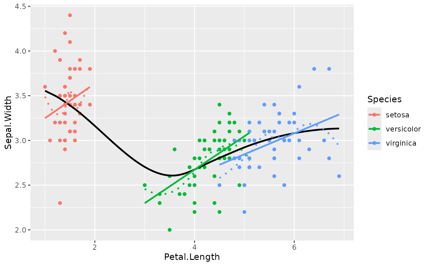
# Get an idea of the data
ggplot(iris, aes(x = Petal.Length, y = Sepal.Width)) +
geom_point(aes(color = Species)) +
geom_smooth(color = "black", se = FALSE) +
geom_smooth(aes(color = Species), linetype = "dotted", se = FALSE) +
geom_smooth(aes(color = Species), method = "lm", se = FALSE)
#> `geom_smooth()` using method = 'loess' and formula = 'y ~ x'
#> `geom_smooth()` using method = 'loess' and formula = 'y ~ x'
#> `geom_smooth()` using formula = 'y ~ x'
 # Model it
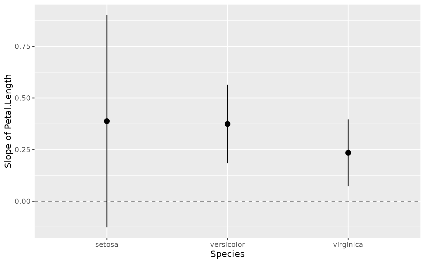
model <- lm(Sepal.Width ~ Species * Petal.Length, data = iris)
# Compute the marginal effect of Petal.Length at each level of Species
slopes <- estimate_slopes(model, slope = "Petal.Length", by = "Species")
slopes
#> Estimated Marginal Effects
#>
#> Species | Slope | SE | 95% CI | t(144) | p
#> -----------------------------------------------------------
#> setosa | 0.39 | 0.26 | [-0.13, 0.90] | 1.49 | 0.138
#> versicolor | 0.37 | 0.10 | [ 0.18, 0.56] | 3.89 | < .001
#> virginica | 0.23 | 0.08 | [ 0.07, 0.40] | 2.86 | 0.005
#>
#> Marginal effects estimated for Petal.Length
#> Type of slope was dY/dX
# What is the *average* slope of Petal.Length? This can be calculated by
# taking the average of the slopes across all Species, using `comparison`.
# We pass a function to `comparison` that calculates the mean of the slopes.
estimate_slopes(
model,
slope = "Petal.Length",
by = "Species",
comparison = ~I(mean(x))
)
#> Estimated Marginal Effects
#>
#> Slope | SE | 95% CI | t(144) | p
#> ---------------------------------------------
#> 0.33 | 0.10 | [0.14, 0.52] | 3.45 | < .001
#>
#> Marginal effects estimated for Petal.Length
# \dontrun{
# Plot it
plot(slopes)
# Model it
model <- lm(Sepal.Width ~ Species * Petal.Length, data = iris)
# Compute the marginal effect of Petal.Length at each level of Species
slopes <- estimate_slopes(model, slope = "Petal.Length", by = "Species")
slopes
#> Estimated Marginal Effects
#>
#> Species | Slope | SE | 95% CI | t(144) | p
#> -----------------------------------------------------------
#> setosa | 0.39 | 0.26 | [-0.13, 0.90] | 1.49 | 0.138
#> versicolor | 0.37 | 0.10 | [ 0.18, 0.56] | 3.89 | < .001
#> virginica | 0.23 | 0.08 | [ 0.07, 0.40] | 2.86 | 0.005
#>
#> Marginal effects estimated for Petal.Length
#> Type of slope was dY/dX
# What is the *average* slope of Petal.Length? This can be calculated by
# taking the average of the slopes across all Species, using `comparison`.
# We pass a function to `comparison` that calculates the mean of the slopes.
estimate_slopes(
model,
slope = "Petal.Length",
by = "Species",
comparison = ~I(mean(x))
)
#> Estimated Marginal Effects
#>
#> Slope | SE | 95% CI | t(144) | p
#> ---------------------------------------------
#> 0.33 | 0.10 | [0.14, 0.52] | 3.45 | < .001
#>
#> Marginal effects estimated for Petal.Length
# \dontrun{
# Plot it
plot(slopes)
 standardize(slopes)
#> Estimated Marginal Effects (standardized)
#>
#> Species | Slope | SE | 95% CI | t(144) | p
#> -----------------------------------------------------------
#> setosa | 0.39 | 0.60 | [-0.29, 2.07] | 1.49 | 0.138
#> versicolor | 0.37 | 0.22 | [ 0.42, 1.30] | 3.89 | < .001
#> virginica | 0.23 | 0.19 | [ 0.17, 0.91] | 2.86 | 0.005
#>
#> Marginal effects estimated for Petal.Length
#> Type of slope was dY/dX
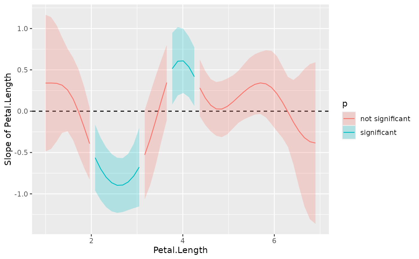
model <- mgcv::gam(Sepal.Width ~ s(Petal.Length), data = iris)
slopes <- estimate_slopes(model, by = "Petal.Length", length = 50)
#> No numeric variable was specified for slope estimation. Selecting `trend
#> = "Petal.Length"`.
summary(slopes)
#> Johnson-Neymann Intervals
#>
#> Start | End | Direction | Confidence
#> ------------------------------------------
#> 1.00 | 1.60 | positive | Not Significant
#> 1.72 | 1.96 | negative | Not Significant
#> 2.08 | 3.05 | negative | Significant
#> 3.17 | 3.41 | negative | Not Significant
#> 3.53 | 3.65 | positive | Not Significant
#> 3.77 | 4.25 | positive | Significant
#> 4.37 | 6.18 | positive | Not Significant
#> 6.30 | 6.90 | negative | Not Significant
#>
#> Marginal effects estimated for Petal.Length
#> Type of slope was dY/dX
plot(slopes)
standardize(slopes)
#> Estimated Marginal Effects (standardized)
#>
#> Species | Slope | SE | 95% CI | t(144) | p
#> -----------------------------------------------------------
#> setosa | 0.39 | 0.60 | [-0.29, 2.07] | 1.49 | 0.138
#> versicolor | 0.37 | 0.22 | [ 0.42, 1.30] | 3.89 | < .001
#> virginica | 0.23 | 0.19 | [ 0.17, 0.91] | 2.86 | 0.005
#>
#> Marginal effects estimated for Petal.Length
#> Type of slope was dY/dX
model <- mgcv::gam(Sepal.Width ~ s(Petal.Length), data = iris)
slopes <- estimate_slopes(model, by = "Petal.Length", length = 50)
#> No numeric variable was specified for slope estimation. Selecting `trend
#> = "Petal.Length"`.
summary(slopes)
#> Johnson-Neymann Intervals
#>
#> Start | End | Direction | Confidence
#> ------------------------------------------
#> 1.00 | 1.60 | positive | Not Significant
#> 1.72 | 1.96 | negative | Not Significant
#> 2.08 | 3.05 | negative | Significant
#> 3.17 | 3.41 | negative | Not Significant
#> 3.53 | 3.65 | positive | Not Significant
#> 3.77 | 4.25 | positive | Significant
#> 4.37 | 6.18 | positive | Not Significant
#> 6.30 | 6.90 | negative | Not Significant
#>
#> Marginal effects estimated for Petal.Length
#> Type of slope was dY/dX
plot(slopes)
 model <- mgcv::gam(Sepal.Width ~ s(Petal.Length, by = Species), data = iris)
slopes <- estimate_slopes(model,
slope = "Petal.Length",
by = c("Petal.Length", "Species"), length = 20
)
summary(slopes)
#> There might be too few data to accurately determine intervals. Consider
#> setting `length = 100` (or larger) in your call to `estimate_slopes()`.
#> Johnson-Neymann Intervals
#>
#> Group | Start | End | Direction | Confidence
#> -------------------------------------------------------
#> setosa | 1.00 | 1.62 | positive | Not Significant
#> versicolor | 3.17 | 5.04 | positive | Significant
#> virginica | 4.73 | 4.73 | positive | Not Significant
#> virginica | 5.04 | 5.66 | positive | Significant
#> virginica | 5.97 | 6.90 | positive | Not Significant
#>
#> Marginal effects estimated for Petal.Length
#> Type of slope was dY/dX
plot(slopes)
model <- mgcv::gam(Sepal.Width ~ s(Petal.Length, by = Species), data = iris)
slopes <- estimate_slopes(model,
slope = "Petal.Length",
by = c("Petal.Length", "Species"), length = 20
)
summary(slopes)
#> There might be too few data to accurately determine intervals. Consider
#> setting `length = 100` (or larger) in your call to `estimate_slopes()`.
#> Johnson-Neymann Intervals
#>
#> Group | Start | End | Direction | Confidence
#> -------------------------------------------------------
#> setosa | 1.00 | 1.62 | positive | Not Significant
#> versicolor | 3.17 | 5.04 | positive | Significant
#> virginica | 4.73 | 4.73 | positive | Not Significant
#> virginica | 5.04 | 5.66 | positive | Significant
#> virginica | 5.97 | 6.90 | positive | Not Significant
#>
#> Marginal effects estimated for Petal.Length
#> Type of slope was dY/dX
plot(slopes)
 # marginal effects, grouped by Species, at different values of Petal.Length
estimate_slopes(model,
slope = "Petal.Length",
by = c("Petal.Length", "Species"), length = 10
)
#> Estimated Marginal Effects
#>
#> Petal.Length | Species | Slope | SE | 95% CI | t(143.68) | p
#> -----------------------------------------------------------------------------
#> 1.00 | setosa | 0.30 | 0.32 | [-0.33, 0.93] | 0.94 | 0.351
#> 1.66 | setosa | 0.22 | 0.24 | [-0.26, 0.70] | 0.90 | 0.370
#> 3.62 | versicolor | 0.38 | 0.10 | [ 0.19, 0.56] | 3.94 | < .001
#> 4.28 | versicolor | 0.38 | 0.10 | [ 0.19, 0.56] | 3.94 | < .001
#> 4.93 | versicolor | 0.38 | 0.10 | [ 0.19, 0.56] | 3.94 | < .001
#> 4.93 | virginica | 0.31 | 0.14 | [ 0.04, 0.58] | 2.23 | 0.027
#> 5.59 | virginica | 0.26 | 0.11 | [ 0.05, 0.47] | 2.42 | 0.017
#> 6.24 | virginica | 0.12 | 0.14 | [-0.16, 0.40] | 0.86 | 0.393
#> 6.90 | virginica | 0.05 | 0.22 | [-0.40, 0.49] | 0.21 | 0.836
#>
#> Marginal effects estimated for Petal.Length
#> Type of slope was dY/dX
# marginal effects at different values of Petal.Length
estimate_slopes(model, slope = "Petal.Length", by = "Petal.Length", length = 10)
#> Estimated Marginal Effects
#>
#> Petal.Length | Slope | SE | 95% CI | t(143.68) | p
#> ------------------------------------------------------------------
#> 1.00 | 0.27 | 0.17 | [-0.06, 0.60] | 1.63 | 0.106
#> 1.66 | 0.25 | 0.13 | [-0.02, 0.51] | 1.86 | 0.066
#> 2.31 | 0.14 | 0.12 | [-0.10, 0.39] | 1.16 | 0.249
#> 2.97 | 0.05 | 0.10 | [-0.15, 0.26] | 0.53 | 0.600
#> 3.62 | 5.50e-03 | 0.11 | [-0.21, 0.22] | 0.05 | 0.959
#> 4.28 | -0.02 | 0.13 | [-0.28, 0.23] | -0.17 | 0.862
#> 4.93 | -0.02 | 0.17 | [-0.36, 0.32] | -0.11 | 0.912
#> 5.59 | -0.05 | 0.22 | [-0.48, 0.38] | -0.22 | 0.825
#> 6.24 | -0.09 | 0.27 | [-0.62, 0.43] | -0.35 | 0.730
#> 6.90 | -0.12 | 0.31 | [-0.73, 0.48] | -0.40 | 0.689
#>
#> Marginal effects estimated for Petal.Length
#> Type of slope was dY/dX
# marginal effects at very specific values of Petal.Length
estimate_slopes(model, slope = "Petal.Length", by = "Petal.Length=c(1, 3, 5)")
#> Estimated Marginal Effects
#>
#> Petal.Length | Slope | SE | 95% CI | t(143.68) | p
#> ---------------------------------------------------------------
#> 1 | 0.27 | 0.17 | [-0.06, 0.60] | 1.63 | 0.106
#> 3 | 0.05 | 0.10 | [-0.16, 0.26] | 0.49 | 0.627
#> 5 | -0.02 | 0.18 | [-0.37, 0.33] | -0.11 | 0.912
#>
#> Marginal effects estimated for Petal.Length
#> Type of slope was dY/dX
# or in "classic" R syntax, using lists
estimate_slopes(model, slope = "Petal.Length", by = list(Petal.Length = c(1, 3, 5)))
#> Estimated Marginal Effects
#>
#> Petal.Length | Slope | SE | 95% CI | t(143.68) | p
#> ---------------------------------------------------------------
#> 1 | 0.27 | 0.17 | [-0.06, 0.60] | 1.63 | 0.106
#> 3 | 0.05 | 0.10 | [-0.16, 0.26] | 0.49 | 0.627
#> 5 | -0.02 | 0.18 | [-0.37, 0.33] | -0.11 | 0.912
#>
#> Marginal effects estimated for Petal.Length
#> Type of slope was dY/dX
# average marginal effects of Petal.Length,
# just for the trend within a certain range
estimate_slopes(model, slope = "Petal.Length=seq(2, 4, 0.01)")
#> Estimated Marginal Effects
#>
#> Slope | SE | 95% CI | t(143.68) | p
#> ------------------------------------------------
#> 0.07 | 0.07 | [-0.08, 0.21] | 0.92 | 0.359
#>
#> Marginal effects estimated for Petal.Length
#> Type of slope was dY/dX
# "classic" R syntax, using lists
estimate_slopes(model, slope = list(Petal.Length = seq(2, 4, 0.01)))
#> Estimated Marginal Effects
#>
#> Slope | SE | 95% CI | t(143.68) | p
#> ------------------------------------------------
#> 0.07 | 0.07 | [-0.08, 0.21] | 0.92 | 0.359
#>
#> Marginal effects estimated for Petal.Length
#> Type of slope was dY/dX
# }
# \dontrun{
# marginal effects with different `estimate` options
data(penguins, package = "datasets")
penguins$long_bill <- factor(datawizard::categorize(penguins$bill_len), labels = c("short", "long"))
m <- glm(long_bill ~ sex + species + island * bill_dep, data = penguins, family = "binomial")
# the emmeans default
estimate_slopes(m, "bill_dep", by = "island")
#> Estimated Marginal Effects
#>
#> island | Slope | SE | 95% CI | z | p
#> --------------------------------------------------------------
#> Biscoe | 6.07e-03 | 4.45e-03 | [ 0.00, 0.01] | 1.36 | 0.173
#> Dream | 0.04 | 0.03 | [-0.01, 0.10] | 1.47 | 0.141
#> Torgersen | 5.29e-03 | 0.01 | [-0.02, 0.03] | 0.41 | 0.679
#>
#> Marginal effects estimated for bill_dep
#> Type of slope was dY/dX
emmeans::emtrends(m, "island", var = "bill_dep", regrid = "response")
#> island bill_dep.trend SE df asymp.LCL asymp.UCL
#> Biscoe 0.00606 0.00445 Inf -0.00267 0.0148
#> Dream 0.04180 0.02830 Inf -0.01372 0.0973
#> Torgersen 0.00528 0.01270 Inf -0.01958 0.0301
#>
#> Results are averaged over the levels of: sex, species
#> Confidence level used: 0.95
# the marginaleffects default
estimate_slopes(m, "bill_dep", by = "island", estimate = "average")
#> Estimated Marginal Effects
#>
#> island | Slope | SE | 95% CI | z | p
#> -------------------------------------------------------
#> Biscoe | 0.06 | 0.04 | [-0.01, 0.14] | 1.75 | 0.079
#> Dream | 0.05 | 0.02 | [ 0.00, 0.10] | 1.93 | 0.053
#> Torgersen | 0.03 | 0.03 | [-0.02, 0.08] | 1.08 | 0.279
#>
#> Marginal effects estimated for bill_dep
#> Type of slope was dY/dX
marginaleffects::avg_slopes(m, variables = "bill_dep", by = "island")
#>
#> island Estimate Std. Error z Pr(>|z|) S 2.5 % 97.5 %
#> Biscoe 0.0640 0.0365 1.75 0.0794 3.7 -0.007509 0.1356
#> Dream 0.0473 0.0245 1.93 0.0534 4.2 -0.000698 0.0952
#> Torgersen 0.0297 0.0274 1.08 0.2786 1.8 -0.024004 0.0833
#>
#> Term: bill_dep
#> Type: response
#> Comparison: dY/dX
#>
# filter by groups
estimate_slopes(m, "bill_dep", by = "island=c('Biscoe','Dream')")
#> Estimated Marginal Effects
#>
#> island | Slope | SE | 95% CI | z | p
#> -----------------------------------------------------------
#> Biscoe | 6.07e-03 | 4.45e-03 | [ 0.00, 0.01] | 1.36 | 0.173
#> Dream | 0.04 | 0.03 | [-0.01, 0.10] | 1.47 | 0.141
#>
#> Marginal effects estimated for bill_dep
#> Type of slope was dY/dX
# or in "classic" R syntax, using lists
estimate_slopes(m, "bill_dep", by = list(island = c('Biscoe', 'Dream')))
#> Estimated Marginal Effects
#>
#> island | Slope | SE | 95% CI | z | p
#> -----------------------------------------------------------
#> Biscoe | 6.07e-03 | 4.45e-03 | [ 0.00, 0.01] | 1.36 | 0.173
#> Dream | 0.04 | 0.03 | [-0.01, 0.10] | 1.47 | 0.141
#>
#> Marginal effects estimated for bill_dep
#> Type of slope was dY/dX
# }
# marginal effects, grouped by Species, at different values of Petal.Length
estimate_slopes(model,
slope = "Petal.Length",
by = c("Petal.Length", "Species"), length = 10
)
#> Estimated Marginal Effects
#>
#> Petal.Length | Species | Slope | SE | 95% CI | t(143.68) | p
#> -----------------------------------------------------------------------------
#> 1.00 | setosa | 0.30 | 0.32 | [-0.33, 0.93] | 0.94 | 0.351
#> 1.66 | setosa | 0.22 | 0.24 | [-0.26, 0.70] | 0.90 | 0.370
#> 3.62 | versicolor | 0.38 | 0.10 | [ 0.19, 0.56] | 3.94 | < .001
#> 4.28 | versicolor | 0.38 | 0.10 | [ 0.19, 0.56] | 3.94 | < .001
#> 4.93 | versicolor | 0.38 | 0.10 | [ 0.19, 0.56] | 3.94 | < .001
#> 4.93 | virginica | 0.31 | 0.14 | [ 0.04, 0.58] | 2.23 | 0.027
#> 5.59 | virginica | 0.26 | 0.11 | [ 0.05, 0.47] | 2.42 | 0.017
#> 6.24 | virginica | 0.12 | 0.14 | [-0.16, 0.40] | 0.86 | 0.393
#> 6.90 | virginica | 0.05 | 0.22 | [-0.40, 0.49] | 0.21 | 0.836
#>
#> Marginal effects estimated for Petal.Length
#> Type of slope was dY/dX
# marginal effects at different values of Petal.Length
estimate_slopes(model, slope = "Petal.Length", by = "Petal.Length", length = 10)
#> Estimated Marginal Effects
#>
#> Petal.Length | Slope | SE | 95% CI | t(143.68) | p
#> ------------------------------------------------------------------
#> 1.00 | 0.27 | 0.17 | [-0.06, 0.60] | 1.63 | 0.106
#> 1.66 | 0.25 | 0.13 | [-0.02, 0.51] | 1.86 | 0.066
#> 2.31 | 0.14 | 0.12 | [-0.10, 0.39] | 1.16 | 0.249
#> 2.97 | 0.05 | 0.10 | [-0.15, 0.26] | 0.53 | 0.600
#> 3.62 | 5.50e-03 | 0.11 | [-0.21, 0.22] | 0.05 | 0.959
#> 4.28 | -0.02 | 0.13 | [-0.28, 0.23] | -0.17 | 0.862
#> 4.93 | -0.02 | 0.17 | [-0.36, 0.32] | -0.11 | 0.912
#> 5.59 | -0.05 | 0.22 | [-0.48, 0.38] | -0.22 | 0.825
#> 6.24 | -0.09 | 0.27 | [-0.62, 0.43] | -0.35 | 0.730
#> 6.90 | -0.12 | 0.31 | [-0.73, 0.48] | -0.40 | 0.689
#>
#> Marginal effects estimated for Petal.Length
#> Type of slope was dY/dX
# marginal effects at very specific values of Petal.Length
estimate_slopes(model, slope = "Petal.Length", by = "Petal.Length=c(1, 3, 5)")
#> Estimated Marginal Effects
#>
#> Petal.Length | Slope | SE | 95% CI | t(143.68) | p
#> ---------------------------------------------------------------
#> 1 | 0.27 | 0.17 | [-0.06, 0.60] | 1.63 | 0.106
#> 3 | 0.05 | 0.10 | [-0.16, 0.26] | 0.49 | 0.627
#> 5 | -0.02 | 0.18 | [-0.37, 0.33] | -0.11 | 0.912
#>
#> Marginal effects estimated for Petal.Length
#> Type of slope was dY/dX
# or in "classic" R syntax, using lists
estimate_slopes(model, slope = "Petal.Length", by = list(Petal.Length = c(1, 3, 5)))
#> Estimated Marginal Effects
#>
#> Petal.Length | Slope | SE | 95% CI | t(143.68) | p
#> ---------------------------------------------------------------
#> 1 | 0.27 | 0.17 | [-0.06, 0.60] | 1.63 | 0.106
#> 3 | 0.05 | 0.10 | [-0.16, 0.26] | 0.49 | 0.627
#> 5 | -0.02 | 0.18 | [-0.37, 0.33] | -0.11 | 0.912
#>
#> Marginal effects estimated for Petal.Length
#> Type of slope was dY/dX
# average marginal effects of Petal.Length,
# just for the trend within a certain range
estimate_slopes(model, slope = "Petal.Length=seq(2, 4, 0.01)")
#> Estimated Marginal Effects
#>
#> Slope | SE | 95% CI | t(143.68) | p
#> ------------------------------------------------
#> 0.07 | 0.07 | [-0.08, 0.21] | 0.92 | 0.359
#>
#> Marginal effects estimated for Petal.Length
#> Type of slope was dY/dX
# "classic" R syntax, using lists
estimate_slopes(model, slope = list(Petal.Length = seq(2, 4, 0.01)))
#> Estimated Marginal Effects
#>
#> Slope | SE | 95% CI | t(143.68) | p
#> ------------------------------------------------
#> 0.07 | 0.07 | [-0.08, 0.21] | 0.92 | 0.359
#>
#> Marginal effects estimated for Petal.Length
#> Type of slope was dY/dX
# }
# \dontrun{
# marginal effects with different `estimate` options
data(penguins, package = "datasets")
penguins$long_bill <- factor(datawizard::categorize(penguins$bill_len), labels = c("short", "long"))
m <- glm(long_bill ~ sex + species + island * bill_dep, data = penguins, family = "binomial")
# the emmeans default
estimate_slopes(m, "bill_dep", by = "island")
#> Estimated Marginal Effects
#>
#> island | Slope | SE | 95% CI | z | p
#> --------------------------------------------------------------
#> Biscoe | 6.07e-03 | 4.45e-03 | [ 0.00, 0.01] | 1.36 | 0.173
#> Dream | 0.04 | 0.03 | [-0.01, 0.10] | 1.47 | 0.141
#> Torgersen | 5.29e-03 | 0.01 | [-0.02, 0.03] | 0.41 | 0.679
#>
#> Marginal effects estimated for bill_dep
#> Type of slope was dY/dX
emmeans::emtrends(m, "island", var = "bill_dep", regrid = "response")
#> island bill_dep.trend SE df asymp.LCL asymp.UCL
#> Biscoe 0.00606 0.00445 Inf -0.00267 0.0148
#> Dream 0.04180 0.02830 Inf -0.01372 0.0973
#> Torgersen 0.00528 0.01270 Inf -0.01958 0.0301
#>
#> Results are averaged over the levels of: sex, species
#> Confidence level used: 0.95
# the marginaleffects default
estimate_slopes(m, "bill_dep", by = "island", estimate = "average")
#> Estimated Marginal Effects
#>
#> island | Slope | SE | 95% CI | z | p
#> -------------------------------------------------------
#> Biscoe | 0.06 | 0.04 | [-0.01, 0.14] | 1.75 | 0.079
#> Dream | 0.05 | 0.02 | [ 0.00, 0.10] | 1.93 | 0.053
#> Torgersen | 0.03 | 0.03 | [-0.02, 0.08] | 1.08 | 0.279
#>
#> Marginal effects estimated for bill_dep
#> Type of slope was dY/dX
marginaleffects::avg_slopes(m, variables = "bill_dep", by = "island")
#>
#> island Estimate Std. Error z Pr(>|z|) S 2.5 % 97.5 %
#> Biscoe 0.0640 0.0365 1.75 0.0794 3.7 -0.007509 0.1356
#> Dream 0.0473 0.0245 1.93 0.0534 4.2 -0.000698 0.0952
#> Torgersen 0.0297 0.0274 1.08 0.2786 1.8 -0.024004 0.0833
#>
#> Term: bill_dep
#> Type: response
#> Comparison: dY/dX
#>
# filter by groups
estimate_slopes(m, "bill_dep", by = "island=c('Biscoe','Dream')")
#> Estimated Marginal Effects
#>
#> island | Slope | SE | 95% CI | z | p
#> -----------------------------------------------------------
#> Biscoe | 6.07e-03 | 4.45e-03 | [ 0.00, 0.01] | 1.36 | 0.173
#> Dream | 0.04 | 0.03 | [-0.01, 0.10] | 1.47 | 0.141
#>
#> Marginal effects estimated for bill_dep
#> Type of slope was dY/dX
# or in "classic" R syntax, using lists
estimate_slopes(m, "bill_dep", by = list(island = c('Biscoe', 'Dream')))
#> Estimated Marginal Effects
#>
#> island | Slope | SE | 95% CI | z | p
#> -----------------------------------------------------------
#> Biscoe | 6.07e-03 | 4.45e-03 | [ 0.00, 0.01] | 1.36 | 0.173
#> Dream | 0.04 | 0.03 | [-0.01, 0.10] | 1.47 | 0.141
#>
#> Marginal effects estimated for bill_dep
#> Type of slope was dY/dX
# }