Interrupted Time Series Analysis • modelbased

Introduction

Interrupted Time Series (ITS) analysis is a powerful quasi-experimental design used to evaluate the effects of an intervention, policy change, or event. The core idea is to study a sequence of observations on an outcome over time, both before and after a specific intervention. By modeling the trend before the intervention, we can create a counterfactual scenario of what would have happened if the intervention had not occurred. Comparing this counterfactual to the actual trend observed after the intervention allows us to estimate the intervention’s impact.

Two key effects are typically of interest in an ITS analysis:

Level Change: An immediate, abrupt change in the outcome right after the intervention.
Slope Change: A change in the trend or rate of change of the outcome following the intervention.

The modelbased package provides an intuitive and powerful set of tools to estimate, test, and visualize these effects. This vignette will walk you through a complete example of an ITS analysis.

Setup and Data Simulation

First, let’s load the necessary package. We’ll use modelbased for the analysis.

library(modelbased)

To demonstrate the method, we will simulate a dataset. Our time series will have 365 time points (e.g., days). A known intervention occurs at day 200.

set.seed(1234)

# Total number of days
n <- 365

# The day the event/intervention starts
event_start <- 200

# Time index from 1 to 365
time <- seq_len(n)

# Event variable: 0 before the intervention and 1 after
event <- c(rep_len(0, event_start), rep_len(1, n - event_start))

Now, we’ll generate our outcome variable. The formula below explicitly defines the pre- and post-intervention dynamics:

# Outcome equation
outcome <-
  10 +                 # 1. Pre-intervention intercept
  15 * time +          # 2. Pre-intervention slope (trend)
  20 * event +         # 3. Level change (a jump of +20)
  5 * event * time +   # 4. Slope change (slope becomes 15 + 5 = 20)
  rnorm(n, mean = 0, sd = 100) # Add some random noise

dat <- data.frame(outcome, time, event)

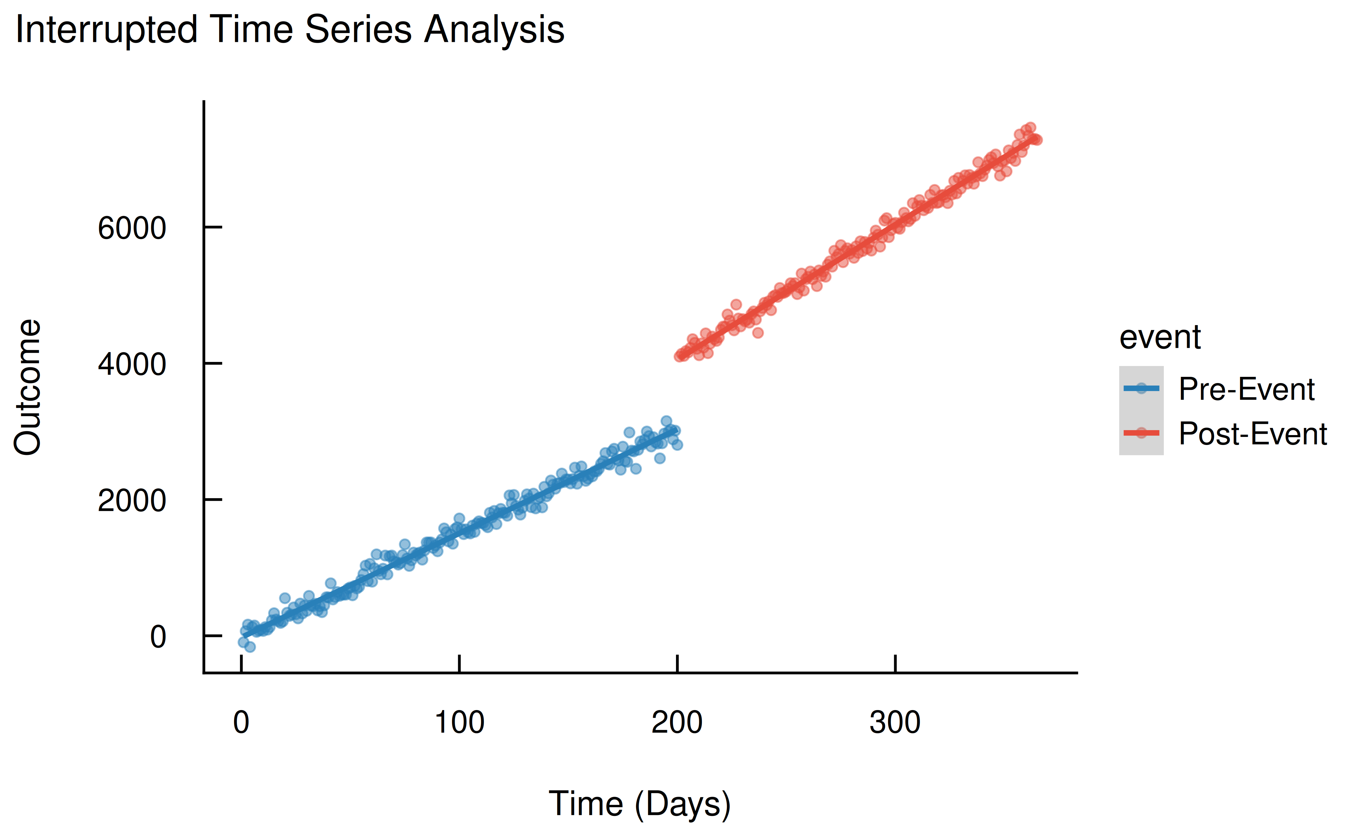
Modeling the Time Series

The standard approach to modeling a simple ITS is with a linear model. The key is to include the time variable, the event variable, and their interaction.

time: Models the underlying trend.
event: Models the immediate level change.
time:event: Models the change in trend (slope) after the intervention.

mod <- lm(outcome ~ time * event, data = dat)

Analyzing the Intervention Effects

With our model fitted, we can now use modelbased to quantify and test the intervention’s effects.

1. The Interruption: Level Change

First, let’s examine what the model estimates for the outcome right before and right after the intervention at time = 200. We can use estimate_means() to get the predicted values at time = 199 and time = 200 for both the factual (event = 1) and counterfactual (event = 0) scenarios.

estimate_means(mod, by = c("time=c(199,200)", "event"))
#> Estimated Marginal Means
#> 
#> time | event |                  Mean (CI)
#> -----------------------------------------
#> 199  |     0 | 3016.42 (2989.26, 3043.59)
#> 200  |     0 | 3031.70 (3004.33, 3059.07)
#> 199  |     1 | 4035.72 (4005.05, 4066.38)
#> 200  |     1 | 4055.53 (4025.14, 4085.92)
#> 
#> Variable predicted: outcome
#> Predictors modulated: time=c(199,200), event

To directly test if the immediate “jump” or “level change” at the moment of the intervention is statistically significant, we can use estimate_contrasts(). We ask for the difference between event = 1 and event = 0 specifically at time = 200.

estimate_contrasts(mod, contrast = "event", by = "time=200")
#> Marginal Contrasts Analysis
#> 
#> Level1 | Level2 | time |           Difference (CI) |      p
#> -----------------------------------------------------------
#> 1      | 0      |  200 | 1023.83 (982.94, 1064.73) | <0.001
#> 
#> Variable predicted: outcome
#> Predictors contrasted: event
#> p-values are uncorrected.

The output shows a large, statistically significant difference of about 1020. This is our estimated level change. It represents the immediate impact of the intervention.

2. The Change in Trend: Slope Change

Next, we want to know if the intervention changed the long-term trend of the outcome. We can use estimate_slopes() to compute the slope of time for the pre-intervention period (event = 0) and the post-intervention period (event = 1).

estimate_slopes(mod, trend = "time", by = "event")
#> Estimated Marginal Effects
#> 
#> event |           Slope (CI) |      p
#> -------------------------------------
#> 0     | 15.28 (15.04, 15.51) | <0.001
#> 1     | 19.82 (19.50, 20.13) | <0.001
#> 
#> Marginal effects estimated for time
#> Type of slope was dY/dX

The results show the pre-intervention slope was around 15, while the post-intervention slope was around 20. But is this difference statistically significant? We can again use estimate_contrasts(), this time contrasting the slopes of time across the levels of event.

estimate_contrasts(mod, contrast = "time", by = "event")
#> Marginal Contrasts Analysis
#> 
#> Level1 | Level2 |   Difference (CI) |      p
#> --------------------------------------------
#> 1      | 0      | 4.54 (4.14, 4.94) | <0.001
#> 
#> Variable predicted: outcome
#> Predictors contrasted: time
#> Predictors averaged: time (1.8e+02)
#> p-values are uncorrected.

The result is a significant difference of approximately 5. This is our estimated slope change. It tells us that after the intervention, the outcome not only jumped to a new level but also started increasing at a significantly faster rate.

Conclusion

This vignette demonstrates how the modelbased package can be used to conduct a comprehensive Interrupted Time Series analysis. By combining a simple linear model with the estimate_means(), estimate_slopes(), and estimate_contrasts() functions, we can easily estimate and test for both immediate (level) and sustained (slope) changes following an intervention. This workflow provides a clear, powerful, and interpretable approach to evaluating the impact of real-world events.