Model-based predictions — estimate_expectation • modelbased

After fitting a model, it is useful generate model-based estimates of the response variables for different combinations of predictor values. Such estimates can be used to make inferences about relationships between variables, to make predictions about individual cases, or to compare the predicted values against the observed data.

The modelbased package includes 4 "related" functions, that mostly differ in their default arguments (in particular, data and predict):

estimate_prediction(data = NULL, predict = "prediction", ...)
estimate_expectation(data = NULL, predict = "expectation", ...)
estimate_relation(data = "grid", predict = "expectation", ...)
estimate_link(data = "grid", predict = "link", ...)

While they are all based on model-based predictions (using insight::get_predicted()), they differ in terms of the type of predictions they make by default. For instance, estimate_prediction() and estimate_expectation() return predictions for the original data used to fit the model, while estimate_relation() and estimate_link() return predictions on a insight::get_datagrid(). Similarly, estimate_link returns predictions on the link scale, while the others return predictions on the response scale. Note that the relevance of these differences depends on the model family (for instance, for linear models, estimate_relation is equivalent to estimate_link(), since there is no difference between the link-scale and the response scale).

Note that you can run plot() on the output of these functions to get some visual insights (see the plotting examples).

See the details section below for details about the different possibilities.

Usage

estimate_expectation(
  model,
  data = NULL,
  by = NULL,
  predict = "expectation",
  ci = 0.95,
  transform = NULL,
  keep_iterations = FALSE,
  ...
)

estimate_link(
  model,
  data = "grid",
  by = NULL,
  predict = "link",
  ci = 0.95,
  transform = NULL,
  keep_iterations = FALSE,
  ...
)

estimate_prediction(
  model,
  data = NULL,
  by = NULL,
  predict = "prediction",
  ci = 0.95,
  transform = NULL,
  keep_iterations = FALSE,
  ...
)

estimate_relation(
  model,
  data = "grid",
  by = NULL,
  predict = "expectation",
  ci = 0.95,
  transform = NULL,
  keep_iterations = FALSE,
  ...
)

Arguments

model: A statistical model.
data: A data frame with model's predictors to estimate the response. If NULL, the model's data is used. If "grid", the model matrix is obtained (through insight::get_datagrid()).
by: The predictor variable(s) at which to estimate the response. Other predictors of the model that are not included here will be set to their mean value (for numeric predictors), reference level (for factors) or mode (other types). The by argument will be used to create a data grid via insight::get_datagrid(), which will then be used as data argument. Thus, you cannot specify both data and by but only of these two arguments.
predict: This parameter controls what is predicted (and gets internally passed to insight::get_predicted()). In most cases, you don't need to care about it: it is changed automatically according to the different predicting functions (i.e., estimate_expectation(), estimate_prediction(), estimate_link() or estimate_relation()). The only time you might be interested in manually changing it is to estimate other distributional parameters (called "dpar" in other packages) - for instance when using complex formulae in brms models. The predict argument can then be set to the parameter you want to estimate, for instance "sigma", "kappa", etc. Note that the distinction between "expectation", "link" and "prediction" does not then apply (as you are directly predicting the value of some distributional parameter), and the corresponding functions will then only differ in the default value of their data argument.
ci: Confidence Interval (CI) level. Default to 0.95 (95%).
transform: A function applied to predictions and confidence intervals to (back-) transform results, which can be useful in case the regression model has a transformed response variable (e.g., lm(log(y) ~ x)). Can also be TRUE, in which case insight::get_transformation() is called to determine the appropriate transformation-function. Note: Standard errors are not (back-) transformed!
keep_iterations: If TRUE, will keep all iterations (draws) of bootstrapped or Bayesian models. They will be added as additional columns named iter_1, iter_2, .... You can reshape them to a long format by running reshape_iterations().
...: You can add all the additional control arguments from insight::get_datagrid() (used when data = "grid") and insight::get_predicted().

Value

A data frame of predicted values and uncertainty intervals, with class "estimate_predicted". Methods for visualisation_recipe() and plot() are available.

Note

These functions are built on top of insight::get_predicted() and correspond to different specifications of its parameters. It may be useful to read its documentation, in particular the description of the predict argument for additional details on the difference between expected vs. predicted values and link vs. response scales.

Additional control parameters can be used to control results from insight::get_datagrid() (when data = "grid") and from insight::get_predicted() (the function used internally to compute predictions).

For plotting, check the examples in visualisation_recipe(). Also check out the Vignettes and README examples for various examples, tutorials and usecases.

Expected (average) values

The most important way that various types of response estimates differ is in terms of what quantity is being estimated and the meaning of the uncertainty intervals. The major choices are expected values for uncertainty in the regression line and predicted values for uncertainty in the individual case predictions.

Expected values refer to the fitted regression line - the estimated average response value (i.e., the "expectation") for individuals with specific predictor values. For example, in a linear model y = 2 + 3x + 4z + e, the estimated average y for individuals with x = 1 and z = 2 is 11.

For expected values, uncertainty intervals refer to uncertainty in the estimated conditional average (where might the true regression line actually fall)? Uncertainty intervals for expected values are also called "confidence intervals".

Expected values and their uncertainty intervals are useful for describing the relationship between variables and for describing how precisely a model has been estimated.

For generalized linear models, expected values are reported on one of two scales:

The link scale refers to scale of the fitted regression line, after transformation by the link function. For example, for a logistic regression (logit binomial) model, the link scale gives expected log-odds. For a log-link Poisson model, the link scale gives the expected log-count.
The response scale refers to the original scale of the response variable (i.e., without any link function transformation). Expected values on the link scale are back-transformed to the original response variable metric (e.g., expected probabilities for binomial models, expected counts for Poisson models).

Individual case predictions

In contrast to expected values, predicted values refer to predictions for individual cases. Predicted values are also called "posterior predictions" or "posterior predictive draws".

For predicted values, uncertainty intervals refer to uncertainty in the individual response values for each case (where might any single case actually fall)? Uncertainty intervals for predicted values are also called "prediction intervals" or "posterior predictive intervals".

Predicted values and their uncertainty intervals are useful for forecasting the range of values that might be observed in new data, for making decisions about individual cases, and for checking if model predictions are reasonable ("posterior predictive checks").

Predicted values and intervals are always on the scale of the original response variable (not the link scale).

Functions for estimating predicted values and uncertainty

modelbased provides 4 functions for generating model-based response estimates and their uncertainty:

estimate_expectation():
- Generates expected values (conditional average) on the response scale.
- The uncertainty interval is a confidence interval.
- By default, values are computed using the data used to fit the model.
estimate_link():
- Generates expected values (conditional average) on the link scale.
- The uncertainty interval is a confidence interval.
- By default, values are computed using a reference grid spanning the observed range of predictor values (see insight::get_datagrid()).
estimate_prediction():
- Generates predicted values (for individual cases) on the response scale.
- The uncertainty interval is a prediction interval.
- By default, values are computed using the data used to fit the model.
estimate_relation():
- Like estimate_expectation().
- Useful for visualizing a model.
- Generates expected values (conditional average) on the response scale.
- The uncertainty interval is a confidence interval.
- By default, values are computed using a reference grid spanning the observed range of predictor values (see insight::get_datagrid()).

Data for predictions

If the data = NULL, values are estimated using the data used to fit the model. If data = "grid", values are computed using a reference grid spanning the observed range of predictor values with insight::get_datagrid(). This can be useful for model visualization. The number of predictor values used for each variable can be controlled with the length argument. data can also be a data frame containing columns with names matching the model frame (see insight::get_data()). This can be used to generate model predictions for specific combinations of predictor values.

Examples

library(modelbased)

# Linear Models
model <- lm(mpg ~ wt, data = mtcars)

# Get predicted and prediction interval (see insight::get_predicted)
estimate_expectation(model)
#> Model-based Predictions
#> 
#> wt   | Predicted |   SE |         95% CI | Residuals
#> ----------------------------------------------------
#> 2.62 |     23.28 | 0.63 | [21.99, 24.58] |     -2.28
#> 2.88 |     21.92 | 0.57 | [20.75, 23.09] |     -0.92
#> 2.32 |     24.89 | 0.74 | [23.38, 26.39] |     -2.09
#> 3.21 |     20.10 | 0.54 | [19.00, 21.20] |      1.30
#> 3.44 |     18.90 | 0.55 | [17.77, 20.03] |     -0.20
#> 3.46 |     18.79 | 0.56 | [17.66, 19.93] |     -0.69
#> 3.57 |     18.21 | 0.57 | [17.03, 19.38] |     -3.91
#> 3.19 |     20.24 | 0.54 | [19.14, 21.34] |      4.16
#> 3.15 |     20.45 | 0.54 | [19.35, 21.55] |      2.35
#> 3.44 |     18.90 | 0.55 | [17.77, 20.03] |      0.30
#> 3.44 |     18.90 | 0.55 | [17.77, 20.03] |     -1.10
#> 4.07 |     15.53 | 0.72 | [14.06, 17.00] |      0.87
#> 3.73 |     17.35 | 0.61 | [16.10, 18.60] |     -0.05
#> 3.78 |     17.08 | 0.62 | [15.81, 18.36] |     -1.88
#> 5.25 |      9.23 | 1.26 | [ 6.66, 11.80] |      1.17
#> 5.42 |      8.30 | 1.35 | [ 5.55, 11.05] |      2.10
#> 5.34 |      8.72 | 1.31 | [ 6.05, 11.39] |      5.98
#> 2.20 |     25.53 | 0.78 | [23.93, 27.13] |      6.87
#> 1.61 |     28.65 | 1.05 | [26.52, 30.79] |      1.75
#> 1.83 |     27.48 | 0.94 | [25.55, 29.40] |      6.42
#> 2.46 |     24.11 | 0.68 | [22.72, 25.51] |     -2.61
#> 3.52 |     18.47 | 0.56 | [17.32, 19.63] |     -2.97
#> 3.44 |     18.93 | 0.55 | [17.80, 20.05] |     -3.73
#> 3.84 |     16.76 | 0.64 | [15.45, 18.07] |     -3.46
#> 3.85 |     16.74 | 0.64 | [15.42, 18.05] |      2.46
#> 1.94 |     26.94 | 0.90 | [25.11, 28.77] |      0.36
#> 2.14 |     25.85 | 0.81 | [24.20, 27.50] |      0.15
#> 1.51 |     29.20 | 1.09 | [26.96, 31.43] |      1.20
#> 3.17 |     20.34 | 0.54 | [19.24, 21.44] |     -4.54
#> 2.77 |     22.48 | 0.59 | [21.27, 23.69] |     -2.78
#> 3.57 |     18.21 | 0.57 | [17.03, 19.38] |     -3.21
#> 2.78 |     22.43 | 0.59 | [21.22, 23.64] |     -1.03
#> 
#> Variable predicted: mpg
#> 

# Get expected values with confidence interval
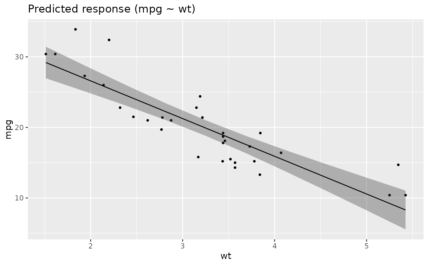
pred <- estimate_relation(model)
pred
#> Model-based Predictions
#> 
#> wt   | Predicted |   SE |         95% CI
#> ----------------------------------------
#> 1.51 |     29.20 | 1.09 | [26.96, 31.43]
#> 1.95 |     26.87 | 0.89 | [25.05, 28.69]
#> 2.38 |     24.55 | 0.71 | [23.10, 26.01]
#> 2.82 |     22.23 | 0.58 | [21.04, 23.42]
#> 3.25 |     19.91 | 0.54 | [18.81, 21.01]
#> 3.69 |     17.59 | 0.60 | [16.36, 18.81]
#> 4.12 |     15.27 | 0.74 | [13.76, 16.77]
#> 4.55 |     12.94 | 0.92 | [11.06, 14.82]
#> 4.99 |     10.62 | 1.13 | [ 8.32, 12.92]
#> 5.42 |      8.30 | 1.35 | [ 5.55, 11.05]
#> 
#> Variable predicted: mpg
#> Predictors modulated: wt
#> 

# Visualisation (see visualisation_recipe())
plot(pred)


# Standardize predictions
pred <- estimate_relation(lm(mpg ~ wt + am, data = mtcars))
z <- standardize(pred, include_response = FALSE)
z
#> Model-based Predictions (standardized)
#> 
#> wt    |    am | Predicted |   SE |         95% CI
#> -------------------------------------------------
#> -1.74 | -0.81 |     29.22 | 1.91 | [25.31, 33.14]
#> -1.30 | -0.81 |     26.89 | 1.60 | [23.62, 30.17]
#> -0.85 | -0.81 |     24.57 | 1.30 | [21.90, 27.24]
#> -0.41 | -0.81 |     22.24 | 1.03 | [20.13, 24.36]
#> 0.03  | -0.81 |     19.92 | 0.82 | [18.24, 21.60]
#> 0.48  | -0.81 |     17.59 | 0.71 | [16.13, 19.05]
#> 0.92  | -0.81 |     15.27 | 0.76 | [13.71, 16.83]
#> 1.37  | -0.81 |     12.94 | 0.94 | [11.01, 14.87]
#> 1.81  | -0.81 |     10.62 | 1.20 | [ 8.17, 13.06]
#> 2.26  | -0.81 |      8.29 | 1.49 | [ 5.25, 11.33]
#> -1.74 |  1.19 |     29.20 | 1.11 | [26.92, 31.48]
#> -1.30 |  1.19 |     26.87 | 0.93 | [24.96, 28.78]
#> -0.85 |  1.19 |     24.55 | 0.86 | [22.79, 26.31]
#> -0.41 |  1.19 |     22.22 | 0.92 | [20.34, 24.09]
#> 0.03  |  1.19 |     19.90 | 1.08 | [17.68, 22.11]
#> 0.48  |  1.19 |     17.57 | 1.32 | [14.86, 20.27]
#> 0.92  |  1.19 |     15.24 | 1.60 | [11.98, 18.51]
#> 1.37  |  1.19 |     12.92 | 1.90 | [ 9.04, 16.79]
#> 1.81  |  1.19 |     10.59 | 2.21 | [ 6.08, 15.11]
#> 2.26  |  1.19 |      8.26 | 2.53 | [ 3.10, 13.43]
#> 
#> Variable predicted: mpg
#> Predictors modulated: wt, am
#> 
unstandardize(z, include_response = FALSE)
#> Model-based Predictions (standardized)
#> 
#> wt   | am | Predicted |   SE |         95% CI
#> ---------------------------------------------
#> 1.51 |  0 |     29.22 | 1.91 | [25.31, 33.14]
#> 1.95 |  0 |     26.89 | 1.60 | [23.62, 30.17]
#> 2.38 |  0 |     24.57 | 1.30 | [21.90, 27.24]
#> 2.82 |  0 |     22.24 | 1.03 | [20.13, 24.36]
#> 3.25 |  0 |     19.92 | 0.82 | [18.24, 21.60]
#> 3.69 |  0 |     17.59 | 0.71 | [16.13, 19.05]
#> 4.12 |  0 |     15.27 | 0.76 | [13.71, 16.83]
#> 4.55 |  0 |     12.94 | 0.94 | [11.01, 14.87]
#> 4.99 |  0 |     10.62 | 1.20 | [ 8.17, 13.06]
#> 5.42 |  0 |      8.29 | 1.49 | [ 5.25, 11.33]
#> 1.51 |  1 |     29.20 | 1.11 | [26.92, 31.48]
#> 1.95 |  1 |     26.87 | 0.93 | [24.96, 28.78]
#> 2.38 |  1 |     24.55 | 0.86 | [22.79, 26.31]
#> 2.82 |  1 |     22.22 | 0.92 | [20.34, 24.09]
#> 3.25 |  1 |     19.90 | 1.08 | [17.68, 22.11]
#> 3.69 |  1 |     17.57 | 1.32 | [14.86, 20.27]
#> 4.12 |  1 |     15.24 | 1.60 | [11.98, 18.51]
#> 4.55 |  1 |     12.92 | 1.90 | [ 9.04, 16.79]
#> 4.99 |  1 |     10.59 | 2.21 | [ 6.08, 15.11]
#> 5.42 |  1 |      8.26 | 2.53 | [ 3.10, 13.43]
#> 
#> Variable predicted: mpg
#> Predictors modulated: wt, am
#> 

# Logistic Models
model <- glm(vs ~ wt, data = mtcars, family = "binomial")
estimate_expectation(model)
#> Model-based Predictions
#> 
#> wt   | Predicted |   SE |       95% CI | Residuals
#> --------------------------------------------------
#> 2.62 |      0.67 | 0.12 | [0.40, 0.86] |     -0.67
#> 2.88 |      0.56 | 0.12 | [0.33, 0.76] |     -0.56
#> 2.32 |      0.78 | 0.12 | [0.47, 0.94] |      0.22
#> 3.21 |      0.39 | 0.11 | [0.21, 0.61] |      0.61
#> 3.44 |      0.30 | 0.11 | [0.14, 0.53] |     -0.30
#> 3.46 |      0.29 | 0.10 | [0.13, 0.53] |      0.71
#> 3.57 |      0.25 | 0.10 | [0.10, 0.50] |     -0.25
#> 3.19 |      0.41 | 0.11 | [0.22, 0.62] |      0.59
#> 3.15 |      0.42 | 0.11 | [0.24, 0.64] |      0.58
#> 3.44 |      0.30 | 0.11 | [0.14, 0.53] |      0.70
#> 3.44 |      0.30 | 0.11 | [0.14, 0.53] |      0.70
#> 4.07 |      0.11 | 0.08 | [0.02, 0.39] |     -0.11
#> 3.73 |      0.20 | 0.10 | [0.07, 0.46] |     -0.20
#> 3.78 |      0.18 | 0.10 | [0.06, 0.45] |     -0.18
#> 5.25 |      0.01 | 0.02 | [0.00, 0.24] |     -0.01
#> 5.42 |  9.49e-03 | 0.02 | [0.00, 0.23] | -9.49e-03
#> 5.34 |      0.01 | 0.02 | [0.00, 0.23] |     -0.01
#> 2.20 |      0.82 | 0.12 | [0.49, 0.96] |      0.18
#> 1.61 |      0.93 | 0.07 | [0.58, 0.99] |      0.07
#> 1.83 |      0.90 | 0.09 | [0.55, 0.99] |      0.10
#> 2.46 |      0.73 | 0.13 | [0.44, 0.91] |      0.27
#> 3.52 |      0.27 | 0.10 | [0.11, 0.51] |     -0.27
#> 3.44 |      0.30 | 0.11 | [0.14, 0.53] |     -0.30
#> 3.84 |      0.16 | 0.10 | [0.05, 0.43] |     -0.16
#> 3.85 |      0.16 | 0.10 | [0.05, 0.43] |     -0.16
#> 1.94 |      0.88 | 0.10 | [0.54, 0.98] |      0.12
#> 2.14 |      0.84 | 0.11 | [0.50, 0.96] |     -0.84
#> 1.51 |      0.94 | 0.07 | [0.60, 0.99] |      0.06
#> 3.17 |      0.42 | 0.11 | [0.23, 0.63] |     -0.42
#> 2.77 |      0.60 | 0.12 | [0.36, 0.80] |     -0.60
#> 3.57 |      0.25 | 0.10 | [0.10, 0.50] |     -0.25
#> 2.78 |      0.60 | 0.12 | [0.36, 0.80] |      0.40
#> 
#> Variable predicted: vs
#> Predictions are on the response-scale.
#> 
estimate_relation(model)
#> Model-based Predictions
#> 
#> wt   | Predicted |   SE |       95% CI
#> --------------------------------------
#> 1.51 |      0.94 | 0.07 | [0.60, 0.99]
#> 1.95 |      0.88 | 0.10 | [0.53, 0.98]
#> 2.38 |      0.76 | 0.12 | [0.46, 0.92]
#> 2.82 |      0.58 | 0.12 | [0.35, 0.78]
#> 3.25 |      0.38 | 0.11 | [0.20, 0.60]
#> 3.69 |      0.21 | 0.10 | [0.07, 0.47]
#> 4.12 |      0.10 | 0.08 | [0.02, 0.38]
#> 4.55 |      0.05 | 0.05 | [0.01, 0.32]
#> 4.99 |      0.02 | 0.03 | [0.00, 0.27]
#> 5.42 |  9.49e-03 | 0.02 | [0.00, 0.23]
#> 
#> Variable predicted: vs
#> Predictors modulated: wt
#> Predictions are on the response-scale.
#> 

# Mixed models
model <- lme4::lmer(mpg ~ wt + (1 | gear), data = mtcars)
estimate_expectation(model)
#> Model-based Predictions
#> 
#> wt   | gear | Predicted |   SE |         95% CI | Residuals
#> -----------------------------------------------------------
#> 2.62 | 4.00 |     24.04 | 0.97 | [22.07, 26.02] |     -3.04
#> 2.88 | 4.00 |     22.76 | 0.93 | [20.86, 24.65] |     -1.76
#> 2.32 | 4.00 |     25.56 | 1.04 | [23.42, 27.70] |     -2.76
#> 3.21 | 3.00 |     19.64 | 0.92 | [17.77, 21.52] |      1.76
#> 3.44 | 3.00 |     18.51 | 0.94 | [16.59, 20.42] |      0.19
#> 3.46 | 3.00 |     18.41 | 0.94 | [16.48, 20.33] |     -0.31
#> 3.57 | 3.00 |     17.85 | 0.96 | [15.89, 19.81] |     -3.55
#> 3.19 | 4.00 |     21.17 | 0.91 | [19.30, 23.04] |      3.23
#> 3.15 | 4.00 |     21.37 | 0.91 | [19.50, 23.24] |      1.43
#> 3.44 | 4.00 |     19.91 | 0.94 | [17.99, 21.83] |     -0.71
#> 3.44 | 4.00 |     19.91 | 0.94 | [17.99, 21.83] |     -2.11
#> 4.07 | 3.00 |     15.33 | 1.10 | [13.08, 17.58] |      1.07
#> 3.73 | 3.00 |     17.04 | 0.99 | [15.01, 19.08] |      0.26
#> 3.78 | 3.00 |     16.79 | 1.01 | [14.73, 18.86] |     -1.59
#> 5.25 | 3.00 |      9.37 | 1.64 | [ 6.01, 12.74] |      1.03
#> 5.42 | 3.00 |      8.50 | 1.74 | [ 4.94, 12.06] |      1.90
#> 5.34 | 3.00 |      8.90 | 1.70 | [ 5.42, 12.37] |      5.80
#> 2.20 | 4.00 |     26.16 | 1.08 | [23.94, 28.38] |      6.24
#> 1.61 | 4.00 |     29.11 | 1.32 | [26.40, 31.82] |      1.29
#> 1.83 | 4.00 |     28.00 | 1.23 | [25.49, 30.51] |      5.90
#> 2.46 | 3.00 |     23.42 | 1.00 | [21.37, 25.48] |     -1.92
#> 3.52 | 3.00 |     18.10 | 0.95 | [16.16, 20.05] |     -2.60
#> 3.44 | 3.00 |     18.53 | 0.94 | [16.61, 20.45] |     -3.33
#> 3.84 | 3.00 |     16.49 | 1.02 | [14.39, 18.59] |     -3.19
#> 3.85 | 3.00 |     16.46 | 1.03 | [14.36, 18.56] |      2.74
#> 1.94 | 4.00 |     27.50 | 1.18 | [25.08, 29.92] |     -0.20
#> 2.14 | 5.00 |     24.65 | 1.10 | [22.39, 26.91] |      1.35
#> 1.51 | 5.00 |     27.81 | 1.37 | [25.01, 30.62] |      2.59
#> 3.17 | 5.00 |     19.45 | 0.91 | [17.58, 21.33] |     -3.65
#> 2.77 | 5.00 |     21.47 | 0.94 | [19.55, 23.40] |     -1.77
#> 3.57 | 5.00 |     17.44 | 0.96 | [15.47, 19.40] |     -2.44
#> 2.78 | 4.00 |     23.24 | 0.94 | [21.32, 25.16] |     -1.84
#> 
#> Variable predicted: mpg
#> 
estimate_relation(model)
#> Model-based Predictions
#> 
#> wt   | gear | Predicted |   SE |         95% CI
#> -----------------------------------------------
#> 1.51 | 0.00 |     28.56 | 1.37 | [25.75, 31.37]
#> 1.95 | 0.00 |     26.36 | 1.18 | [23.95, 28.78]
#> 2.38 | 0.00 |     24.17 | 1.03 | [22.07, 26.27]
#> 2.82 | 0.00 |     21.98 | 0.93 | [20.07, 23.89]
#> 3.25 | 0.00 |     19.79 | 0.92 | [17.91, 21.67]
#> 3.69 | 0.00 |     17.59 | 0.98 | [15.58, 19.61]
#> 4.12 | 0.00 |     15.40 | 1.12 | [13.12, 17.69]
#> 4.55 | 0.00 |     13.21 | 1.30 | [10.55, 15.87]
#> 4.99 | 0.00 |     11.02 | 1.51 | [ 7.93, 14.11]
#> 5.42 | 0.00 |      8.83 | 1.74 | [ 5.27, 12.39]
#> 
#> Variable predicted: mpg
#> Predictors modulated: wt
#> 

# Bayesian models
# \donttest{
model <- suppressWarnings(rstanarm::stan_glm(
  mpg ~ wt,
  data = mtcars, refresh = 0, iter = 200
))
estimate_expectation(model)
#> Model-based Predictions
#> 
#> wt   | Predicted |   SE |         95% CI | Residuals
#> ----------------------------------------------------
#> 2.62 |     23.46 | 0.78 | [22.19, 25.03] |     -2.46
#> 2.88 |     22.10 | 0.70 | [20.96, 23.67] |     -1.10
#> 2.32 |     25.06 | 0.91 | [23.52, 26.96] |     -2.26
#> 3.21 |     20.28 | 0.65 | [19.09, 21.84] |      1.12
#> 3.44 |     19.08 | 0.66 | [17.92, 20.61] |     -0.38
#> 3.46 |     18.98 | 0.66 | [17.80, 20.50] |     -0.88
#> 3.57 |     18.39 | 0.68 | [17.17, 19.90] |     -4.09
#> 3.19 |     20.42 | 0.65 | [19.22, 21.93] |      3.98
#> 3.15 |     20.63 | 0.65 | [19.42, 22.15] |      2.17
#> 3.44 |     19.08 | 0.66 | [17.92, 20.61] |      0.12
#> 3.44 |     19.08 | 0.66 | [17.92, 20.61] |     -1.28
#> 4.07 |     15.72 | 0.84 | [14.20, 17.52] |      0.68
#> 3.73 |     17.54 | 0.72 | [16.26, 19.18] |     -0.24
#> 3.78 |     17.27 | 0.73 | [15.97, 18.91] |     -2.07
#> 5.25 |      9.43 | 1.46 | [ 6.81, 12.51] |      0.97
#> 5.42 |      8.50 | 1.57 | [ 5.70, 11.81] |      1.90
#> 5.34 |      8.92 | 1.52 | [ 6.20, 12.16] |      5.78
#> 2.20 |     25.70 | 0.97 | [24.07, 27.76] |      6.70
#> 1.61 |     28.82 | 1.28 | [26.59, 31.47] |      1.58
#> 1.83 |     27.65 | 1.16 | [25.71, 30.10] |      6.25
#> 2.46 |     24.29 | 0.84 | [22.91, 26.01] |     -2.79
#> 3.52 |     18.66 | 0.67 | [17.46, 20.16] |     -3.16
#> 3.44 |     19.11 | 0.66 | [17.95, 20.65] |     -3.91
#> 3.84 |     16.95 | 0.75 | [15.65, 18.57] |     -3.65
#> 3.85 |     16.92 | 0.75 | [15.63, 18.54] |      2.28
#> 1.94 |     27.11 | 1.10 | [25.26, 29.44] |      0.19
#> 2.14 |     26.02 | 1.00 | [24.34, 28.11] |     -0.02
#> 1.51 |     29.36 | 1.34 | [27.00, 32.13] |      1.04
#> 3.17 |     20.52 | 0.65 | [19.33, 22.04] |     -4.72
#> 2.77 |     22.66 | 0.73 | [21.46, 24.23] |     -2.96
#> 3.57 |     18.39 | 0.68 | [17.17, 19.90] |     -3.39
#> 2.78 |     22.60 | 0.73 | [21.42, 24.17] |     -1.20
#> 
#> Variable predicted: mpg
#> 
estimate_relation(model)
#> Model-based Predictions
#> 
#> wt   | Predicted |   SE |         95% CI
#> ----------------------------------------
#> 1.51 |     29.36 | 1.34 | [27.00, 32.13]
#> 1.95 |     27.04 | 1.10 | [25.20, 29.35]
#> 2.38 |     24.73 | 0.88 | [23.26, 26.55]
#> 2.82 |     22.41 | 0.72 | [21.27, 23.98]
#> 3.25 |     20.09 | 0.65 | [18.91, 21.69]
#> 3.69 |     17.77 | 0.70 | [16.55, 19.38]
#> 4.12 |     15.46 | 0.86 | [13.91, 17.28]
#> 4.55 |     13.13 | 1.07 | [11.29, 15.28]
#> 4.99 |     10.82 | 1.31 | [ 8.49, 13.55]
#> 5.42 |      8.50 | 1.57 | [ 5.70, 11.81]
#> 
#> Variable predicted: mpg
#> Predictors modulated: wt
#> 
# }