An Introduction to Growth Mixture Models with brms and easystats

Introduction

Growth Mixture Models (GMMs) are a powerful statistical technique used to identify unobserved subgroups (latent classes) within a population that exhibit different developmental trajectories over time. They are a subclass of latent class analysis and are particularly useful in longitudinal research to understand heterogeneity in how individuals change.

This vignette demonstrates how to conduct a Growth Mixture Model using the brms package for Bayesian modeling and the easystats ecosystem (particularly modelbased, parameters, and see) for easy interpretation and visualization.

Loading Packages and Data

First, we load the necessary packages. brms is for model fitting, and easystats is a suite of packages that simplifies the entire process of statistical analysis and visualization.

library(easystats)
library(brms)
library(ggplot2)

The Dataset

We will use the qol_cancer dataset, which is included in the datawizard package. This dataset contains longitudinal data on the health-related quality of life (QoL) of cancer patients, measured at three time points: pre-surgery, and 6 and 12 months post-surgery.

The dataset includes the following variables:

ID: A unique identifier for each patient.
QoL: The outcome variable, a Quality of Life score.
time: The measurement time point (1 = pre-surgery, 2 = 6 months, 3 = 12 months).
hospital: The hospital where the operation was performed.
education: The patient’s education level (low, mid, high).
age: The patient’s age (standardized).

Let’s prepare the data by converting the time and hospital variables to factors.

data(qol_cancer)

qol_cancer$time <- as.factor(qol_cancer$time)
qol_cancer$hospital <- as.factor(qol_cancer$hospital)

Fitting the Growth Mixture Model

The core of a GMM in brms is the mixture() family, which allows us to model the outcome variable as a mixture of distributions. In our case, we hypothesize that there are distinct subgroups of patients with different QoL trajectories. We will fit a model with two latent classes (nmix = 2).

The model formula QoL ~ time + hospital + education + age + (1 + time | ID) specifies that QoL is predicted by several fixed effects (time, hospital, etc.) and a random effects structure (1 + time | ID). This random effects part is crucial for growth models, as it allows each patient (ID) to have their own baseline QoL (random intercept 1) and their own rate of change over time (random slope time).

Running the Model

Fitting a Bayesian mixture model can be computationally intensive. For the purposes of this vignette, we will download a pre-fitted model from the easystats repository.

# Download the pre-fitted model
brms_mixture_2 <- download_model("brms_mixture_2")

If you wish to fit the model yourself, you can use the following code. Be aware that it may take several minutes to run.

# In case of convergence issues, specifying priors can help. The priors are
# set for the population-level intercept of each mixture component (mu1, mu2).
# prior <- c(
#   prior(normal(0, 10), class = Intercept, dpar = mu1),
#   prior(normal(0, 10), class = Intercept, dpar = mu2)
# )

set.seed(1234)
brms_mixture_2 <- brms::brm(
  formula = QoL ~ time + hospital + education + age + (1 + time | ID),
  data = qol_cancer,
  family = mixture(gaussian, nmix = 2), # Gaussian mixture with 2 classes
  chains = 4,      # Number of MCMC chains
  iter = 2000,     # Total iterations per chain
  cores = 4,       # Use 4 CPU cores
  seed = 1234,     # For reproducibility
  silent = 2,      # Suppress Stan progress
  refresh = 0
)

You can use different factors to predict the outcome for each group in your data. To do this, simply create a separate prediction formula for each part of your model. For instance, you could use one set of factors to predict the quality of life for “Group 1” and a different set for “Group 2”. You can even use factors to predict which group someone is likely to belong to. While this guide won’t cover the details, a code example at the end shows you how.

Interpreting the Model

With our model fitted, we can now use the easystats functions to understand the results.

Predicted Class Membership

Our first step is to determine which latent class each patient belongs to at each time point. We can use the estimate_prediction() function from the modelbased package with predict = "classification".

out <- estimate_prediction(brms_mixture_2, predict = "classification")
head(out)
#> Model-based Predictions
#> 
#> time | hospital | education |   age | ID | Predicted | Probability
#> ------------------------------------------------------------------
#> 3    | 1        | mid       | -3.60 | 1  |      1.00 |        0.72
#> 1    | 1        | mid       | -3.60 | 1  |      2.00 |        0.51
#> 2    | 1        | mid       | -3.60 | 1  |      1.00 |        0.50
#> 1    | 1        | mid       |  1.40 | 10 |      2.00 |        0.97
#> 2    | 1        | mid       |  1.40 | 10 |      2.00 |        0.97
#> 3    | 1        | mid       |  1.40 | 10 |      2.00 |        0.97
#> 
#> time |       95% CI | Residuals
#> -------------------------------
#> 3    | [0.00, 1.00] |     40.67
#> 1    | [0.00, 1.00] |     39.67
#> 2    | [0.00, 1.00] |     32.33
#> 1    | [0.86, 1.00] |     81.33
#> 2    | [0.85, 1.00] |     81.33
#> 3    | [0.89, 1.00] |     81.33
#> 
#> Variable predicted: QoL
#> Predictions are on the classification-scale.

The output table shows the Predicted class for each observation, along with the Probability of that classification. Now, let’s join these predicted classes back to our original dataset for visualization.

# we also keep ID and time for joining, to match observations in the original dataset
d <- data_join(qol_cancer, out[c("time", "ID", "Predicted")], by = c("ID", "time"))
d$class <- as.factor(d$Predicted)

Visualizing Latent Class Trajectories

Now we can visualize the average QoL trajectories for each latent class. This is the most intuitive way to understand the results of a GMM.

ggplot(d, aes(x = as.numeric(time), y = QoL, color = class, fill = class)) +
  geom_smooth(method = "lm") +
  geom_point(alpha = 0.3, position = position_jitter(width = 0.1)) +
  labs(
    title = "Average Latent Class Trajectories of Quality of Life",
    x = "Time (1=pre-op, 2=6m, 3=12m)",
    y = "Quality of Life (QoL)"
  ) +
  theme_modern(show.ticks = TRUE) +
  scale_color_material() +
  scale_fill_material()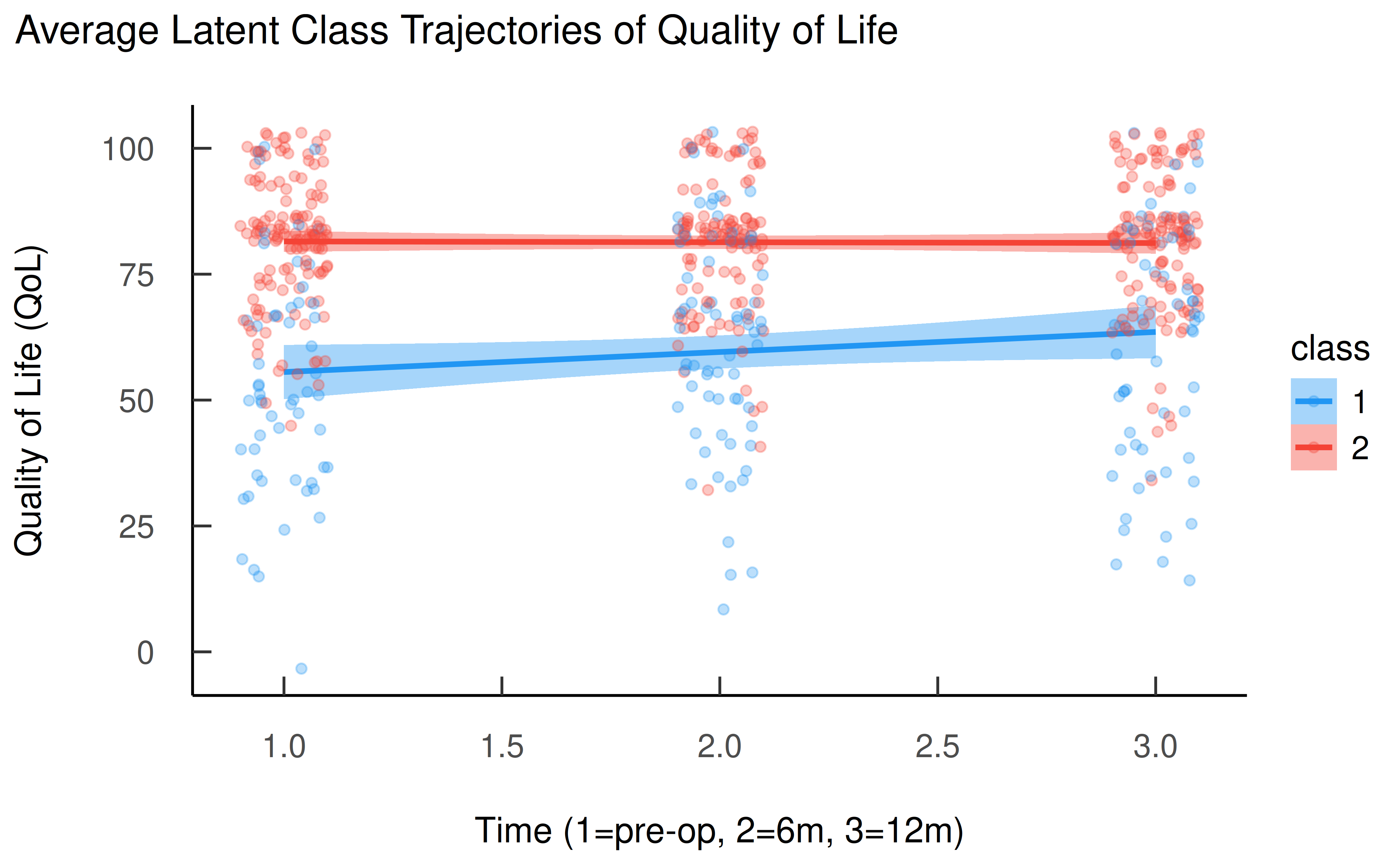

The plot clearly reveals two distinct groups:

Class 1 (blue): This group starts with a lower Quality of Life, but shows a steady improvement over the 12-month period.
Class 2 (red): This group starts with a much higher Quality of Life and maintains this high level throughout the observation period.

Inspecting Model Parameters

To understand what predicts the outcome within each class, we can inspect the model parameters using model_parameters() from the parameters package.

model_parameters(brms_mixture_2, diagnostic = NULL, drop = "time")
#> # Class 1
#> 
#> Parameter     | Median |          95% CI |     pd
#> -------------------------------------------------
#> (Intercept)   |  48.16 | [ 18.63, 63.83] | 99.70%
#> hospital1     |   3.82 | [-17.62, 19.56] | 56.20%
#> educationmid  |   9.32 | [  3.04, 24.36] | 98.65%
#> educationhigh |  13.04 | [ -3.75, 24.99] | 94.10%
#> age           |   0.48 | [ -0.83,  1.20] | 84.00%
#> 
#> # Class 2
#> 
#> Parameter     | Median |          95% CI |     pd
#> -------------------------------------------------
#> (Intercept)   |  75.51 | [ 63.81, 81.50] |   100%
#> hospital1     |  -1.29 | [-10.41,  8.28] | 56.70%
#> educationmid  |   3.98 | [  0.14, 10.17] | 97.65%
#> educationhigh |  11.53 | [  5.79, 19.47] |   100%
#> age           |  -0.37 | [ -0.65,  0.29] | 86.25%

The output is neatly separated by class. We can see, for example, that higher education (educationmid, educationhigh) is associated with a higher QoL in both classes, but the magnitude of the effect differs.

Estimated Marginal Means

We can dive deeper by estimating the marginal means of QoL for different predictor levels within each class. Let’s look at the effect of education. The predict = "link" argument is essential for mixture models, as it computes the means for each class separately.

estimate_means(brms_mixture_2, by = "education", predict = "link")
#> Estimated Marginal Means
#> 
#> education |          Median (CI) | pd   | Class
#> -----------------------------------------------
#> low       | 53.92 (33.41, 63.72) | 100% |     1
#> low       | 74.43 (67.38, 78.20) | 100% |     2
#> mid       | 64.11 (49.39, 72.54) | 100% |     1
#> mid       | 79.19 (73.50, 82.46) | 100% |     2
#> high      | 63.10 (44.67, 76.24) | 100% |     1
#> high      | 86.32 (79.66, 93.25) | 100% |     2
#> 
#> Variable predicted: QoL
#> Predictors modulated: education
#> Predictors averaged: time, hospital, age (0.22), ID
#> Predictions are on the link-scale.

This table gives us the expected mean QoL for each education level, conditional on class membership. For instance, a patient with “low” education in Class 2 has an estimated mean QoL of 74.43, whereas a similar patient in Class 1 has an estimated mean QoL of 53.92.

Comparing Levels with Contrasts

We can also compute contrasts between predictor levels to understand the magnitude of differences.

If we compute contrasts without predict = "link", estimate_contrasts() averages the effects across both classes, giving a general sense of inequality.

estimate_contrasts(
  brms_mixture_2,
  contrast = "education"
)
#> Marginal Contrasts Analysis
#> 
#> Level1 | Level2 |         Median (CI) |     pd
#> ----------------------------------------------
#> mid    | low    |  7.95 (2.60, 11.32) | 99.65%
#> high   | low    | 12.69 (7.17, 17.13) |   100%
#> high   | mid    |  5.67 (1.02,  8.57) | 98.95%
#> 
#> Variable predicted: QoL
#> Predictors contrasted: education
#> Predictors averaged: time, hospital, age (0.22), ID
#> Contrasts are on the response-scale.

More interestingly, we can set predict = "link" to get contrasts both within and between classes. This provides a very detailed picture.

estimate_contrasts(
  brms_mixture_2,
  contrast = "education",
  predict = "link"
)
#> Marginal Contrasts Analysis
#> 
#> Level1 | Level2 |           Median (CI) |     pd
#> ------------------------------------------------
#> 1 mid  | 1 low  |  9.32 (  3.04, 24.36) | 98.65%
#> 1 high | 1 low  | 13.04 ( -3.75, 24.99) | 94.10%
#> 2 low  | 1 low  | 19.34 (  7.55, 40.32) | 99.95%
#> 2 mid  | 1 low  | 27.05 ( 15.71, 44.71) |   100%
#> 2 high | 1 low  | 37.41 ( 23.25, 52.04) |   100%
#> 1 high | 1 mid  |  0.19 (-14.77,  9.54) | 51.20%
#> 2 low  | 1 mid  | 10.00 ( -0.73, 24.01) | 96.80%
#> 2 mid  | 1 mid  | 16.88 (  7.02, 29.15) | 99.45%
#> 2 high | 1 mid  | 24.44 ( 13.22, 35.72) |   100%
#> 2 low  | 1 high | 11.78 ( -1.48, 27.71) | 73.90%
#> 2 mid  | 1 high | 17.61 (  2.51, 32.07) | 99.85%
#> 2 high | 1 high | 24.59 ( 10.05, 39.85) |   100%
#> 2 mid  | 2 low  |  3.98 (  0.14, 10.17) | 97.65%
#> 2 high | 2 low  | 11.53 (  5.79, 19.47) |   100%
#> 2 high | 2 mid  |  7.55 (  3.15, 11.33) | 99.90%
#> 
#> Variable predicted: QoL
#> Predictors contrasted: education
#> Predictors averaged: time, hospital, age (0.22), ID
#> Contrasts are on the link-scale.

The output is rich with information. For example, 2 high | 2 low shows the contrast between high and low education within Class 2 (an increase of 11.53 in QoL), while 2 low | 1 low compares a patient with low education in Class 2 to a patient with low education in Class 1 (a difference of 19.34).

Quantifying Inequality

Finally, estimate_contrasts() has a powerful comparison = "inequality" argument. This calculates the average absolute difference between all levels of a predictor, providing a single number that quantifies the overall disparity associated with that variable. Let’s compare the inequality associated with education versus hospital.

estimate_contrasts(
  brms_mixture_2,
  contrast = c("education", "hospital"),
  comparison = "inequality"
)
#> Marginal Inequality Analysis
#> 
#> Parameter |        Median (CI) |   pd
#> -------------------------------------
#> education | 8.46 (4.85, 11.42) | 100%
#> hospital  | 1.40 (0.11,  8.87) | 100%
#> 
#> Variable predicted: QoL
#> Predictors contrasted: education, hospital
#> Differences are on the response-scale.

The results are striking. The inequality median for education is 8.46, while for hospital it is only 1.40. This suggests that a patient’s education level is associated with far greater disparities in their quality of life trajectory than the hospital where they received treatment.

Conclusion

Growth Mixture Models are an excellent tool for uncovering hidden heterogeneity in longitudinal data. By using brms to fit these complex models and the easystats ecosystem to process and interpret them, researchers can move from complex output to actionable insights with ease. This vignette has shown how to identify latent classes, visualize their trajectories, and quantify the effects of covariates in a straightforward and intuitive workflow.

Supplement

The estimation of latent class membership in finite mixture models within the R package brms is not governed by a single, fixed mechanism. Instead, brms provides a flexible and powerful framework that allows the researcher to explicitly define the data-generating process, including the factors that determine class membership. The central question of whether class membership is determined by the outcome’s trajectory, by predictors, or if predictors are only relevant after classification, can be addressed directly: all of these scenarios represent valid modeling choices that can be implemented within brms. In a mixture model, the probabilities of belonging to each latent class - the mixing proportions, denoted as \theta - are themselves parameters of the model. Consequently, they can be modeled as a function of predictors.

Here’s a summary of how to specify these different scenarios in brms:

Example `brms` Formula Syntax for Common Mixture Model Scenarios
Scenario	Research Question	Example `brms` Formula
Simple Mixture	“Are there two or more distinct latent groups in my outcome data, ignoring all predictors?”	`bf(y ~ 1, family = mixture(gaussian, nmix = 2))`
Predicting Component Means	“Does a treatment (`x`) affect the outcome differently for the two latent groups?”	`bf(y ~ 1, mu1 ~ x, mu2 ~ x, family = mix)` or simply `bf(y ~ x, family = mix)`
Predicting Mixing Proportion	“Does a demographic variable (`z`) predict which latent group an individual is likely to belong to?”	`bf(y ~ 1, theta2 ~ z, family = mix)`
Full Distributional Model	“How do treatment (`x`) and demographics (`z`) jointly influence both the outcome within each group and the probability of group membership?”	`bf(y ~ 1, mu1 ~ x, mu2 ~ x, theta2 ~ z, sigma ~ group, family = mix)`

Example Codes

# this model is actually equivalent to the one we used in the vignette
# but it allows for different predictors for each class
brms::brm(
  bf(
    # formula for individual trajectories
    QoL ~ 1 + (1 + time | ID),
    # predictors for class 1
    mu1 ~ time + hospital + education + age + (1 + time | ID),
    # predictors for class 2
    mu2 ~ time + hospital + education + age + (1 + time | ID),
    family = mixture(gaussian, nmix = 2)
  ),
  data = qol_cancer,
  chains = 4,      # Number of MCMC chains
  iter = 1000,     # Total iterations per chain
  cores = 4,       # Use 4 CPU cores
  seed = 1234,     # For reproducibility
  refresh = 0
)

# in this example, we also model the class membership probabilities
brms::brm(
  bf(
    # formula for individual trajectories
    QoL ~ 1 + (1 + time | ID),
    # predictors for class 1
    mu1 ~ time + hospital + education + age + (1 + time | ID),
    # predictors for class 2
    mu2 ~ time + hospital + education + age + (1 + time | ID),
    # predictors for class membership probabilities
    theta1 ~ hospital + education,
    theta2 ~ hospital + education + age,
    family = mixture(gaussian, nmix = 2)
  ),
  data = qol_cancer,
  chains = 4,      # Number of MCMC chains
  iter = 1000,     # Total iterations per chain
  cores = 4,       # Use 4 CPU cores
  seed = 1234,     # For reproducibility
  refresh = 0
)

The easystats team

2025-06-25