Contrasts and pairwise comparisons

This vignette is the first in a 4-part series:

Contrasts and Pairwise Comparisons
Comparisons of Slopes, Floodlight and Spotlight Analysis (Johnson-Neyman Intervals)
Contrasts and Comparisons for Generalized Linear Models
Contrasts and Comparisons for Zero-Inflation Models

Hypothesis testing for categorical predictors

A reason to compute adjusted predictions (or estimated marginal means) is to help understanding the relationship between predictors and outcome of a regression model. The next step, which often follows this, is to see if there are statistically significant differences. These could be, for example, differences between groups, i.e. between the levels of categorical predictors or whether trends differ significantly from each other.

The modelbased package provides a function, estimate_contrasts(), which does exactly this: testing differences of predictions or marginal means for statistical significance. This is usually called contrasts or (pairwise) comparisons, or marginal effects (if the difference refers to a one-unit change of predictors). This vignette shows some examples how to use the estimate_contrasts() function and how to test whether differences in predictions are statistically significant.

First, different examples for pairwise comparisons are shown, later we will see how to test differences-in-differences (in the emmeans package, also called interaction contrasts).

Within `episode`, do levels differ?

We start with a toy example, where we have a linear model with two categorical predictors. No interaction is involved for now.

We display a simple table of regression coefficients, created with model_parameters() from the parameters package.

library(modelbased)
library(parameters)
library(ggplot2)

set.seed(123)
n <- 200
d <- data.frame(
  outcome = rnorm(n),
  grp = as.factor(sample(c("treatment", "control"), n, TRUE)),
  episode = as.factor(sample(1:3, n, TRUE)),
  sex = as.factor(sample(c("female", "male"), n, TRUE, prob = c(0.4, 0.6)))
)
model1 <- lm(outcome ~ grp + episode, data = d)
model_parameters(model1)
#> Parameter       | Coefficient |   SE |        95% CI | t(196) |     p
#> ---------------------------------------------------------------------
#> (Intercept)     |       -0.08 | 0.13 | [-0.33, 0.18] |  -0.60 | 0.552
#> grp [treatment] |       -0.17 | 0.13 | [-0.44, 0.09] |  -1.30 | 0.197
#> episode [2]     |        0.36 | 0.16 | [ 0.03, 0.68] |   2.18 | 0.031
#> episode [3]     |        0.10 | 0.16 | [-0.22, 0.42] |   0.62 | 0.538

Predictions

Let us look at the adjusted predictions.

my_predictions <- estimate_means(model1, "episode")
my_predictions
#> Estimated Marginal Means
#> 
#> episode |           Mean (CI)
#> -----------------------------
#> 1       | -0.16 (-0.39, 0.07)
#> 2       |  0.20 (-0.04, 0.43)
#> 3       | -0.06 (-0.28, 0.16)
#> 
#> Variable predicted: outcome
#> Predictors modulated: episode
#> Predictors averaged: grp

plot(my_predictions)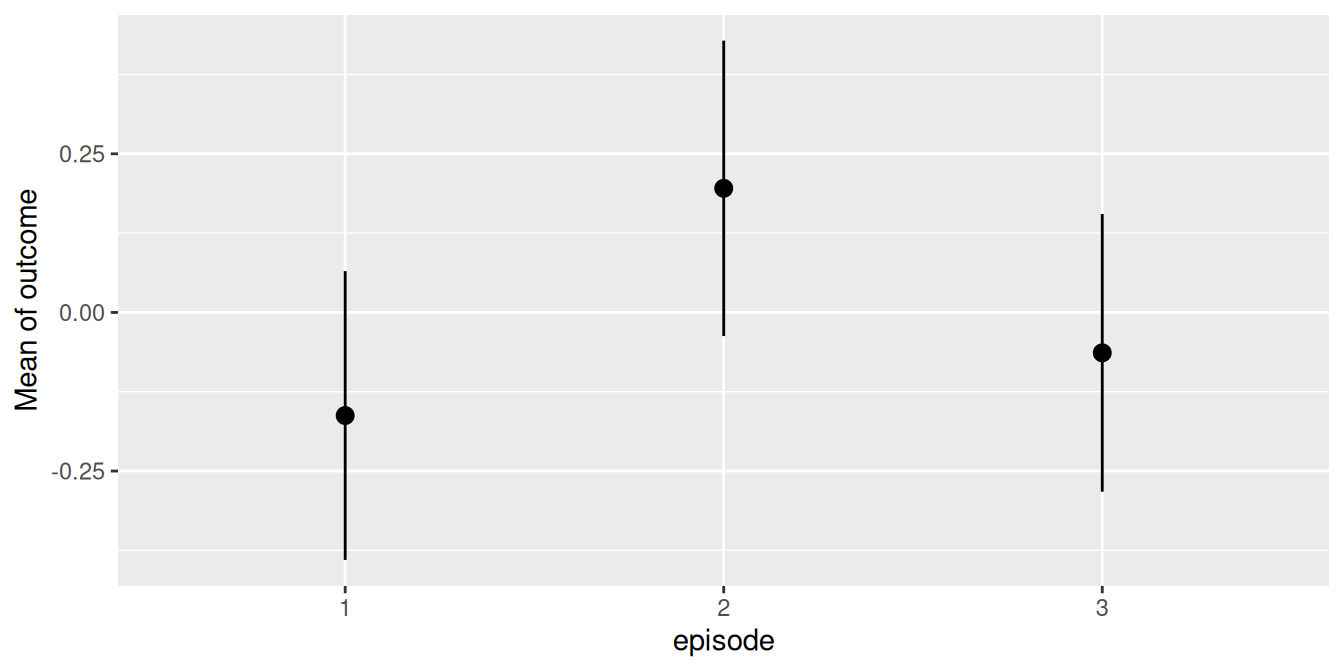

We now see that, for instance, the predicted outcome when espisode = 2 is 0.2.

Pairwise comparisons

We could now ask whether the predicted outcome for episode = 1 is significantly different from the predicted outcome at episode = 2.

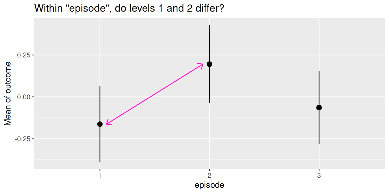
To do this, we use the estimate_contrasts() function. By default, a pairwise comparison is performed. You can specify other comparisons as well, using the comparison argument. For now, we go on with the simpler example of contrasts or pairwise comparisons.

# argument `comparison` defaults to "pairwise"
estimate_contrasts(model1, "episode")
#> Marginal Contrasts Analysis
#> 
#> Level1 | Level2 |     Difference (CI) |     p
#> ---------------------------------------------
#> 2      | 1      |  0.36 ( 0.03, 0.68) | 0.031
#> 3      | 1      |  0.10 (-0.22, 0.42) | 0.538
#> 3      | 2      | -0.26 (-0.58, 0.06) | 0.112
#> 
#> Variable predicted: outcome
#> Predictors contrasted: episode
#> Predictors averaged: grp
#> p-values are uncorrected.

For our quantity of interest, the contrast between episode levels 2 and 1, we see the value 0.36, which is exactly the difference between the predicted outcome for episode = 1 (-0.16) and episode = 2 (0.20). The related p-value is 0.031, indicating that the difference between the predicted values of our outcome at these two levels of the factor episode is indeed statistically significant.

We can also define “representative values” via the contrast or by arguments. For example, we could specify the levels of episode directly, to simplify the output:

estimate_contrasts(model1, contrast = "episode=c(1,2)")
#> Marginal Contrasts Analysis
#> 
#> Level1 | Level2 |   Difference (CI) |     p
#> -------------------------------------------
#> 2      | 1      | 0.36 (0.03, 0.68) | 0.031
#> 
#> Variable predicted: outcome
#> Predictors contrasted: episode=c(1,2)
#> Predictors averaged: grp
#> p-values are uncorrected.

Does same level of episode differ between groups?

The next example includes a pairwise comparison of an interaction between two categorical predictors.

model2 <- lm(outcome ~ grp * episode, data = d)
model_parameters(model2)
#> Parameter                     | Coefficient |   SE |        95% CI | t(194) |     p
#> -----------------------------------------------------------------------------------
#> (Intercept)                   |        0.03 | 0.15 | [-0.27, 0.33] |   0.18 | 0.853
#> grp [treatment]               |       -0.42 | 0.23 | [-0.88, 0.04] |  -1.80 | 0.074
#> episode [2]                   |        0.20 | 0.22 | [-0.23, 0.63] |   0.94 | 0.350
#> episode [3]                   |       -0.07 | 0.22 | [-0.51, 0.37] |  -0.32 | 0.750
#> grp [treatment] × episode [2] |        0.36 | 0.33 | [-0.29, 1.02] |   1.09 | 0.277
#> grp [treatment] × episode [3] |        0.37 | 0.32 | [-0.27, 1.00] |   1.14 | 0.254

Predictions

First, we look at the predicted values of outcome for all combinations of the involved interaction term.

my_predictions <- estimate_means(model2, by = c("episode", "grp"))
my_predictions
#> Estimated Marginal Means
#> 
#> episode | grp       |            Mean (CI)
#> ------------------------------------------
#> 1       | control   |  0.03 (-0.27,  0.33)
#> 2       | control   |  0.23 (-0.08,  0.54)
#> 3       | control   | -0.04 (-0.36,  0.28)
#> 1       | treatment | -0.39 (-0.74, -0.04)
#> 2       | treatment |  0.18 (-0.18,  0.53)
#> 3       | treatment | -0.09 (-0.39,  0.21)
#> 
#> Variable predicted: outcome
#> Predictors modulated: episode, grp

plot(my_predictions)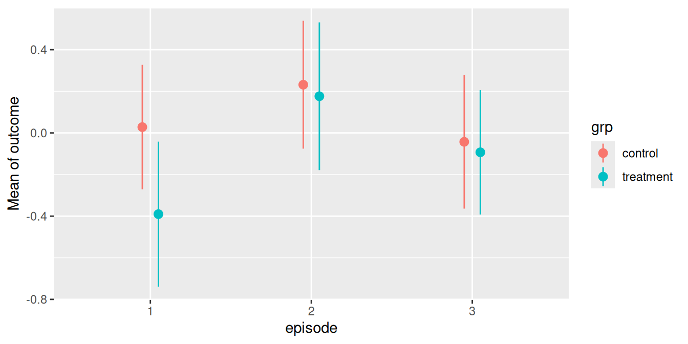

Pairwise comparisons

We could now ask whether the predicted outcome for episode = 2 is significantly different depending on the level of grp? In other words, do the groups treatment and control differ when episode = 2?

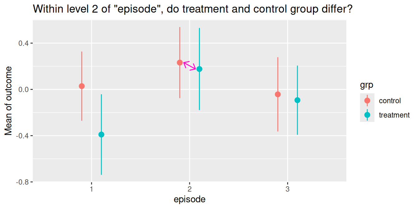
Again, to answer this question, we calculate all pairwise comparisons, i.e. the comparison (or test for differences) between all combinations of our focal predictors. The focal predictors we’re interested here are our two variables used for the interaction.

# we want "episode = 2-2" and "grp = control-treatment"
estimate_contrasts(model2, contrast = c("episode", "grp"))
#> Marginal Contrasts Analysis
#> 
#> Level1       | Level2       |     Difference (CI) |     p
#> ---------------------------------------------------------
#> 1, treatment | 1, control   | -0.42 (-0.88, 0.04) | 0.074
#> 2, control   | 1, control   |  0.20 (-0.23, 0.63) | 0.350
#> 2, treatment | 1, control   |  0.15 (-0.32, 0.61) | 0.529
#> 3, control   | 1, control   | -0.07 (-0.51, 0.37) | 0.750
#> 3, treatment | 1, control   | -0.12 (-0.54, 0.30) | 0.573
#> 2, control   | 1, treatment |  0.62 ( 0.16, 1.09) | 0.009
#> 2, treatment | 1, treatment |  0.57 ( 0.07, 1.06) | 0.026
#> 3, control   | 1, treatment |  0.35 (-0.13, 0.82) | 0.150
#> 3, treatment | 1, treatment |  0.30 (-0.16, 0.76) | 0.203
#> 2, treatment | 2, control   | -0.06 (-0.52, 0.41) | 0.816
#> 3, control   | 2, control   | -0.27 (-0.72, 0.17) | 0.225
#> 3, treatment | 2, control   | -0.32 (-0.75, 0.10) | 0.137
#> 3, control   | 2, treatment | -0.22 (-0.70, 0.26) | 0.368
#> 3, treatment | 2, treatment | -0.27 (-0.73, 0.19) | 0.254
#> 3, treatment | 3, control   | -0.05 (-0.49, 0.39) | 0.821
#> 
#> Variable predicted: outcome
#> Predictors contrasted: episode, grp
#> p-values are uncorrected.

For our quantity of interest, the contrast between groups treatment and control when episode = 2 is 0.35. We find this comparison in row 8 of the above output.

As we can see, estimate_contrasts() returns pairwise comparisons of all possible combinations of factor levels from our focal variables. If we’re only interested in a very specific comparison, we have two options to simplify the output:

We could directly formulate this comparison. Therefore, we need to know the parameters of interests (see below).
We pass specific values or levels to the contrast argument.

Option 1: Directly specify the comparison

estimate_means(model2, by = c("episode", "grp"))
#> Estimated Marginal Means
#> 
#> episode | grp       |            Mean (CI)
#> ------------------------------------------
#> 1       | control   |  0.03 (-0.27,  0.33)
#> 2       | control   |  0.23 (-0.08,  0.54)
#> 3       | control   | -0.04 (-0.36,  0.28)
#> 1       | treatment | -0.39 (-0.74, -0.04)
#> 2       | treatment |  0.18 (-0.18,  0.53)
#> 3       | treatment | -0.09 (-0.39,  0.21)
#> 
#> Variable predicted: outcome
#> Predictors modulated: episode, grp

In the above output, each row is considered as one coefficient of interest. Our groups we want to include in our comparison are rows two (grp = control and episode = 2) and five (grp = treatment and episode = 2), so our “quantities of interest” are b2 and b5. Our null hypothesis we want to test is whether both predictions are equal, i.e. comparison = "b5 = b2" (we could also specify "b2 = b5", results would be the same, just signs are switched). We can now calculate the desired comparison directly:

# compute specific contrast directly
estimate_contrasts(model2, contrast = c("episode", "grp"), comparison = "b2 = b5")
#> Marginal Contrasts Analysis
#> 
#> Parameter |    Difference (CI) |     p
#> --------------------------------------
#> b2=b5     | 0.06 (-0.41, 0.52) | 0.816
#> 
#> Variable predicted: outcome
#> Predictors contrasted: episode, grp
#> p-values are uncorrected.
#> Parameters:
#> b2 = episode [2], grp [control]
#> b5 = episode [2], grp [treatment]

Option 2: Specify values or levels

Again, using representative values for the contrast argument, we can also simplify the output using an alternative syntax:

# return pairwise comparisons for specific values, in
# this case for episode = 2 in both groups
estimate_contrasts(model2, contrast = c("episode=2", "grp"))
#> Marginal Contrasts Analysis
#> 
#> Level1    | Level2  |     Difference (CI) |     p
#> -------------------------------------------------
#> treatment | control | -0.06 (-0.52, 0.41) | 0.816
#> 
#> Variable predicted: outcome
#> Predictors contrasted: episode=2, grp
#> p-values are uncorrected.

This is equivalent to the above example, where we directly specified the comparison we’re interested in. However, the comparison argument might provide more flexibility in case you want more complex comparisons. See examples below.

Do different episode levels differ between groups?

We can repeat the steps shown above to test any combination of group levels for differences.

Pairwise comparisons

For instance, we could now ask whether the predicted outcome for episode = 1 in the treatment group is significantly different from the predicted outcome for episode = 3 in the control group.

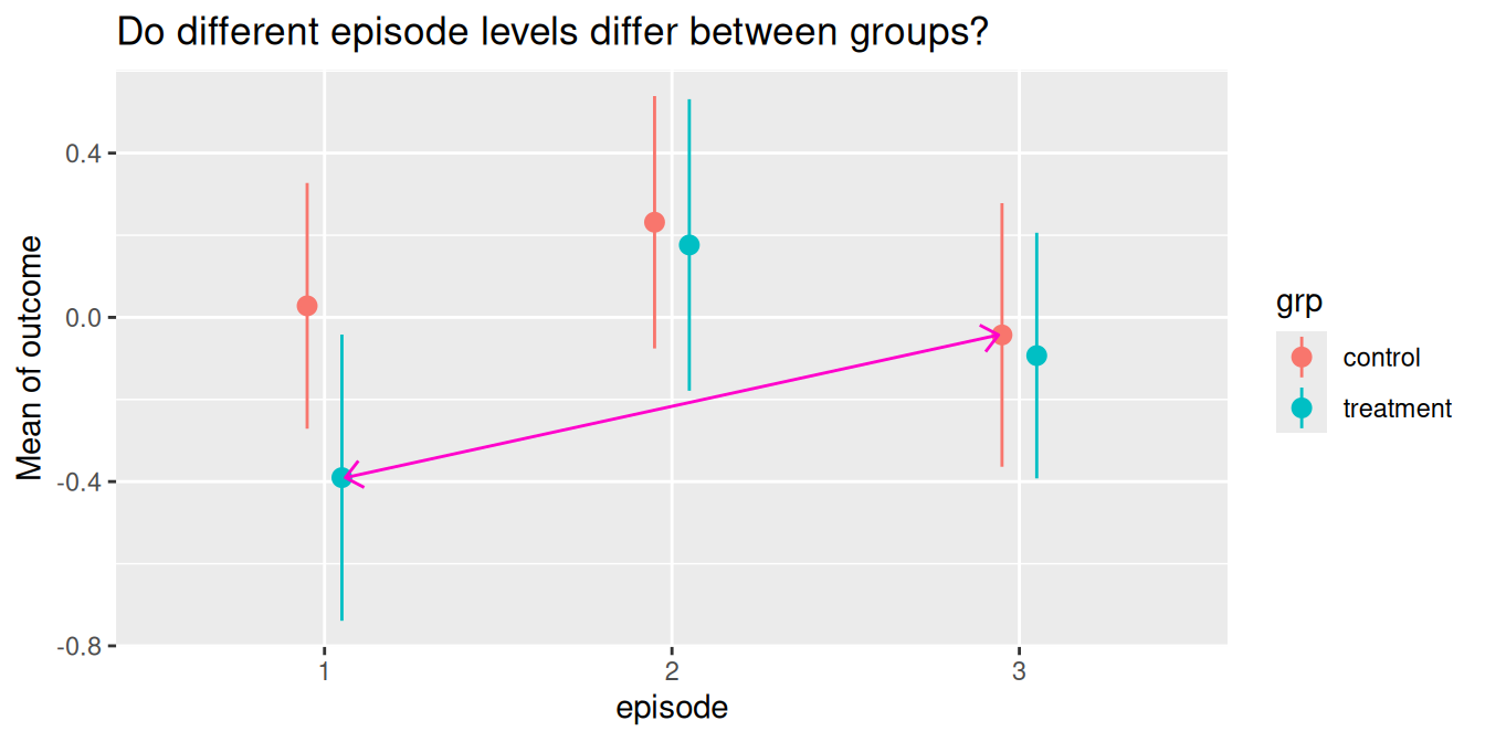
The contrast we are interested in is between episode = 1 in the treatment group and episode = 3 in the control group. These are the predicted values in rows three and four (c.f. above table of predicted values), thus we comparison whether "b4 = b3".

estimate_contrasts(model2, contrast = c("episode", "grp"), comparison = "b4 = b3")
#> Marginal Contrasts Analysis
#> 
#> Parameter |     Difference (CI) |     p
#> ---------------------------------------
#> b4=b3     | -0.35 (-0.82, 0.13) | 0.150
#> 
#> Variable predicted: outcome
#> Predictors contrasted: episode, grp
#> p-values are uncorrected.
#> Parameters:
#> b4 = episode [1], grp [treatment]
#> b3 = episode [3], grp [control]

Another way to produce this pairwise comparison, we can reduce the table of predicted values by providing specific values or levels in the by or contrast argument:

estimate_means(model2, by = c("episode=c(1,3)", "grp"))
#> Estimated Marginal Means
#> 
#> episode | grp       |            Mean (CI)
#> ------------------------------------------
#> 1       | control   |  0.03 (-0.27,  0.33)
#> 3       | control   | -0.04 (-0.36,  0.28)
#> 1       | treatment | -0.39 (-0.74, -0.04)
#> 3       | treatment | -0.09 (-0.39,  0.21)
#> 
#> Variable predicted: outcome
#> Predictors modulated: episode=c(1,3), grp

episode = 1 in the treatment group and episode = 3 in the control group refer now to rows two and three in the reduced output, thus we also can obtain the desired comparison this way:

estimate_contrasts(
  model2,
  contrast = c("episode = c(1, 3)", "grp"),
  comparison = "b3 = b2"
)
#> Marginal Contrasts Analysis
#> 
#> Parameter |     Difference (CI) |     p
#> ---------------------------------------
#> b3=b2     | -0.35 (-0.82, 0.13) | 0.150
#> 
#> Variable predicted: outcome
#> Predictors contrasted: episode = c(1, 3), grp
#> p-values are uncorrected.
#> Parameters:
#> b3 = episode [1], grp [treatment]
#> b2 = episode [3], grp [control]

Does difference between two levels of episode in the control group differ from difference of same two levels in the treatment group?

The comparison argument also allows us to compare difference-in-differences (aka interaction contrasts). For example, is the difference between two episode levels in one group significantly different from the difference of the same two episode levels in the other group?

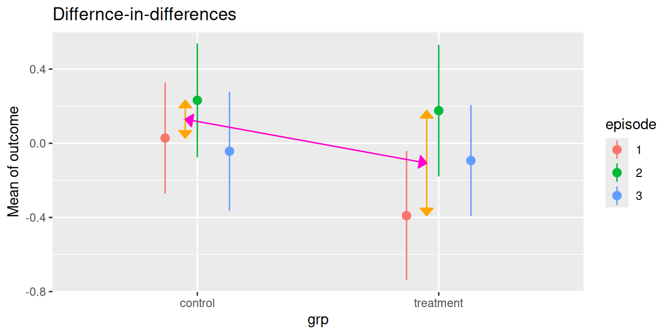
As a reminder, we look at the table of predictions again:

estimate_means(model2, c("episode", "grp"))
#> Estimated Marginal Means
#> 
#> episode | grp       |            Mean (CI)
#> ------------------------------------------
#> 1       | control   |  0.03 (-0.27,  0.33)
#> 2       | control   |  0.23 (-0.08,  0.54)
#> 3       | control   | -0.04 (-0.36,  0.28)
#> 1       | treatment | -0.39 (-0.74, -0.04)
#> 2       | treatment |  0.18 (-0.18,  0.53)
#> 3       | treatment | -0.09 (-0.39,  0.21)
#> 
#> Variable predicted: outcome
#> Predictors modulated: episode, grp

The first difference of episode levels 1 and 2 in the control group refer to rows one and two in the above table (b1 and b2). The difference for the same episode levels in the treatment group refer to the difference between rows four and five (b4 and b5). Thus, we have b1 - b2 and b4 - b5, and our null hypothesis is that these two differences are equal: comparison = "(b1 - b2) = (b4 - b5)".

estimate_contrasts(
  model2,
  c("episode", "grp"),
  comparison = "(b1 - b2) = (b4 - b5)"
)
#> Marginal Contrasts Analysis
#> 
#> Parameter   |    Difference (CI) |     p
#> ----------------------------------------
#> b1-b2=b4-b5 | 0.36 (-0.29, 1.02) | 0.277
#> 
#> Variable predicted: outcome
#> Predictors contrasted: episode, grp
#> p-values are uncorrected.
#> Parameters:
#> b1 = episode [1], grp [control]
#> b2 = episode [2], grp [control]
#> b4 = episode [1], grp [treatment]
#> b5 = episode [2], grp [treatment]

Let’s replicate this step-by-step:

Predicted value of outcome for episode = 1 in the control group is 0.03.
Predicted value of outcome for episode = 2 in the control group is -0.39.
The first difference is 0.42.
Predicted value of outcome for episode = 1 in the treatment group is 0.18.
Predicted value of outcome for episode = 2 in the treatment group is -0.04.
The second difference is 0.22.
Our quantity of interest is the difference between these two differences, which is 0.20. This difference is not statistically significant (p = 0.277).

Conclusion

While the current implementation in estimate_contrasts() already covers many common use cases for testing contrasts and pairwise comparison, there still might be the need for more sophisticated comparisons. In this case, we recommend using the marginaleffects package directly. Some further related recommended readings are the vignettes about Comparisons or Hypothesis Tests.

Go to next vignette: Comparisons of Slopes, Floodlight and Spotlight Analysis (Johnson-Neyman Intervals)

Hypothesis testing for categorical predictors

Within episode, do levels differ?

Predictions

Pairwise comparisons

Does same level of episode differ between groups?

Predictions

Pairwise comparisons

Option 1: Directly specify the comparison

Option 2: Specify values or levels

Do different episode levels differ between groups?

Pairwise comparisons

Does difference between two levels of episode in the control group differ from difference of same two levels in the treatment group?

Conclusion

Within `episode`, do levels differ?