Create a reference grid

Create a reference matrix, useful for visualisation, with evenly spread and combined values. Usually used to generate predictions using get_predicted(). See this vignette for a tutorial on how to create a visualisation matrix using this function.

Alternatively, these can also be used to extract the "grid" columns from objects generated by emmeans and marginaleffects (see those methods for more info).

Usage

get_datagrid(x, ...)

# S3 method for class 'data.frame'
get_datagrid(
  x,
  by = "all",
  factors = "reference",
  numerics = "mean",
  length = 10,
  range = "range",
  preserve_range = FALSE,
  protect_integers = TRUE,
  digits = 3,
  reference = x,
  ...
)

# S3 method for class 'numeric'
get_datagrid(
  x,
  length = 10,
  range = "range",
  protect_integers = TRUE,
  digits = 3,
  ...
)

# S3 method for class 'factor'
get_datagrid(x, ...)

# Default S3 method
get_datagrid(
  x,
  by = "all",
  factors = "reference",
  numerics = "mean",
  preserve_range = TRUE,
  reference = x,
  include_smooth = TRUE,
  include_random = FALSE,
  include_response = FALSE,
  data = NULL,
  digits = 3,
  verbose = TRUE,
  ...
)

Arguments

x

An object from which to construct the reference grid.

...

Arguments passed to or from other methods (for instance, length or range to control the spread of numeric variables.).

by

Indicates the focal predictors (variables) for the reference grid and at which values focal predictors should be represented. If not specified otherwise, representative values for numeric variables or predictors are evenly distributed from the minimum to the maximum, with a total number of length values covering that range (see 'Examples'). Possible options for by are:

Select variables only:
- "all", which will include all variables or predictors.
- a character vector of one or more variable or predictor names, like c("Species", "Sepal.Width"), which will create a grid of all combinations of unique values.
Note: If by specifies only variable names, without associated values, the following occurs: factor variables use all their levels, numeric variables use a range of length equally spaced values between their minimum and maximum, and character variables use all their unique values.
Select variables and values:
- by can be a list of named elements, indicating focal predictors and their representative values, e.g. by = list(mpg = 10:20), by = list(Sepal.Length = c(2, 4), Species = "setosa"), or by = list(Sepal.Length = seq(2, 5, 0.5)).
- Instead of a list, it is possible to write a string representation, or a character vector of such strings, e.g. by = "mpg = 10:20", by = c("Sepal.Length = c(2, 4)", "Species = 'setosa'"), or by = "Sepal.Length = seq(2, 5, 0.5)". Note the usage of single and double quotes to assign strings within strings.
- In general, any expression after a = will be evaluated as R code, which allows using own functions, e.g.
```
fun <- function(x) x^2
get_datagrid(iris, by = "Sepal.Width = fun(2:5)")
```
Note: If by specifies variables with their associated values, argument length is ignored.

There is a special handling of assignments with brackets, i.e. values defined inside [ and ], which create summaries for numeric variables. Following "tokens" that creates pre-defined representative values are possible:

for mean and -/+ 1 SD around the mean: "x = [sd]"
for median and -/+ 1 MAD around the median: "x = [mad]"
for Tukey's five number summary (minimum, lower-hinge, median, upper-hinge, maximum): "x = [fivenum]"
for quartiles: "x = [quartiles]" (same as "x = [fivenum]", but excluding minimum and maximum)
for terciles: "x = [terciles]"
for terciles, including minimum and maximum: "x = [terciles2]"
for a pretty value range: "x = [pretty]"
for minimum and maximum value: "x = [minmax]"
for 0 and the maximum value: "x = [zeromax]"
for a random sample from all values: "x = [sample <number>]", where <number> should be a positive integer, e.g. "x = [sample 15]".

Note: the length argument will be ignored when using brackets-tokens.

The remaining variables not specified in by will be fixed (see also arguments factors and numerics).

factors

Type of summary for factors not specified in by. Can be "reference" (set at the reference level), "mode" (set at the most common level) or "all" to keep all levels.

numerics

Type of summary for numeric values not specified in by. Can be "all" (will duplicate the grid for all unique values), any function ("mean", "median", ...) or a value (e.g., numerics = 0).

length

Length of numeric target variables selected in by (if no representative values are additionally specified). This arguments controls the number of (equally spread) values that will be taken to represent the continuous (non-integer alike!) variables. A longer length will increase precision, but can also substantially increase the size of the datagrid (especially in case of interactions). If NA, will return all the unique values.

In case of multiple continuous target variables, length can also be a vector of different values (see 'Examples'). In this case, length must be of same length as numeric target variables. If length is a named vector, values are matched against the names of the target variables.

When range = "range" (the default), length is ignored for integer type variables when length is larger than the number of unique values and protect_integers is TRUE (default). Set protect_integers = FALSE to create a spread of length number of values from minimum to maximum for integers, including fractions (i.e., to treat integer variables as regular numeric variables).

length is furthermore ignored if "tokens" (in brackets [ and ]) are used in by, or if representative values are additionally specified in by.

range

Option to control the representative values given in by, if no specific values were provided. Use in combination with the length argument to control the number of values within the specified range. range can be one of the following:

"range" (default), will use the minimum and maximum of the original data vector as end-points (min and max). For integer variables, the length argument will be ignored, and "range" will only use values that appear in the data. Set protect_integers = FALSE to override this behaviour for integer variables.
if an interval type is specified, such as "iqr", "ci", "hdi" or "eti", it will spread the values within that range (the default CI width is 95% but this can be changed by adding for instance ci = 0.90.) See IQR() and bayestestR::ci(). This can be useful to have more robust change and skipping extreme values.
if "sd" or "mad", it will spread by this dispersion index around the mean or the median, respectively. If the length argument is an even number (e.g., 4), it will have one more step on the positive side (i.e., -1, 0, +1, +2). The result is a named vector. See 'Examples.'
"grid" will create a reference grid that is useful when plotting predictions, by choosing representative values for numeric variables based on their position in the reference grid. If a numeric variable is the first predictor in by, values from minimum to maximum of the same length as indicated in length are generated. For numeric predictors not specified at first in by, mean and -1/+1 SD around the mean are returned. For factors, all levels are returned.

range can also be a vector of different values (see 'Examples'). In this case, range must be of same length as numeric target variables. If range is a named vector, values are matched against the names of the target variables.

preserve_range

In the case of combinations between numeric variables and factors, setting preserve_range = TRUE will drop the observations where the value of the numeric variable is originally not present in the range of its factor level. This leads to an unbalanced grid. Also, if you want the minimum and the maximum to closely match the actual ranges, you should increase the length argument.

protect_integers

Defaults to TRUE. Indicates whether integers (whole numbers) should be treated as integers (i.e., prevent adding any in-between round number values), or - if FALSE - as regular numeric variables. Only applies when range = "range" (the default), or if range = "grid" and the first predictor in by is an integer.

digits

Number of digits used for rounding numeric values specified in by. E.g., x = [sd] will round the mean and +-/1 SD in the data grid to digits.

reference

The reference vector from which to compute the mean and SD. Used when standardizing or unstandardizing the grid using effectsize::standardize.

include_smooth

If x is a model object, decide whether smooth terms should be included in the data grid or not.

include_random

If x is a mixed model object, decide whether random effect terms should be included in the data grid or not. If include_random is FALSE, but x is a mixed model with random effects, these will still be included in the returned grid, but set to their "population level" value (e.g., NA for glmmTMB or 0 for merMod). This ensures that common predict() methods work properly, as these usually need data with all variables in the model included.

include_response

If x is a model object, decide whether the response variable should be included in the data grid or not.

data

Optional, the data frame that was used to fit the model. Usually, the data is retrieved via get_data().

verbose

Toggle warnings.

Value

Reference grid data frame.

Details

Data grids are an (artificial or theoretical) representation of the sample. They consists of predictors of interest (so-called focal predictors), and meaningful values, at which the sample characteristics (focal predictors) should be represented. The focal predictors are selected in by. To select meaningful (or representative) values, either use by, or use a combination of the arguments length and range.

Examples

# Datagrids of variables and dataframes =====================================
data(iris)
data(mtcars)

# Single variable is of interest; all others are "fixed" ------------------

# Factors, returns all the levels
get_datagrid(iris, by = "Species")
#>      Species Sepal.Length Sepal.Width Petal.Length Petal.Width
#> 1     setosa     5.843333    3.057333        3.758    1.199333
#> 2 versicolor     5.843333    3.057333        3.758    1.199333
#> 3  virginica     5.843333    3.057333        3.758    1.199333
# Specify an expression
get_datagrid(iris, by = "Species = c('setosa', 'versicolor')")
#>      Species Sepal.Length Sepal.Width Petal.Length Petal.Width
#> 1     setosa     5.843333    3.057333        3.758    1.199333
#> 2 versicolor     5.843333    3.057333        3.758    1.199333

# Numeric variables, default spread length = 10
get_datagrid(iris, by = "Sepal.Length")
#>    Sepal.Length Sepal.Width Petal.Length Petal.Width Species
#> 1           4.3    3.057333        3.758    1.199333  setosa
#> 2           4.7    3.057333        3.758    1.199333  setosa
#> 3           5.1    3.057333        3.758    1.199333  setosa
#> 4           5.5    3.057333        3.758    1.199333  setosa
#> 5           5.9    3.057333        3.758    1.199333  setosa
#> 6           6.3    3.057333        3.758    1.199333  setosa
#> 7           6.7    3.057333        3.758    1.199333  setosa
#> 8           7.1    3.057333        3.758    1.199333  setosa
#> 9           7.5    3.057333        3.758    1.199333  setosa
#> 10          7.9    3.057333        3.758    1.199333  setosa
# change length
get_datagrid(iris, by = "Sepal.Length", length = 3)
#>   Sepal.Length Sepal.Width Petal.Length Petal.Width Species
#> 1          4.3    3.057333        3.758    1.199333  setosa
#> 2          6.1    3.057333        3.758    1.199333  setosa
#> 3          7.9    3.057333        3.758    1.199333  setosa

# change non-targets fixing
get_datagrid(iris[2:150, ],
  by = "Sepal.Length",
  factors = "mode", numerics = "median"
)
#>    Sepal.Length Sepal.Width Petal.Length Petal.Width    Species
#> 1           4.3           3          4.4         1.3 versicolor
#> 2           4.7           3          4.4         1.3 versicolor
#> 3           5.1           3          4.4         1.3 versicolor
#> 4           5.5           3          4.4         1.3 versicolor
#> 5           5.9           3          4.4         1.3 versicolor
#> 6           6.3           3          4.4         1.3 versicolor
#> 7           6.7           3          4.4         1.3 versicolor
#> 8           7.1           3          4.4         1.3 versicolor
#> 9           7.5           3          4.4         1.3 versicolor
#> 10          7.9           3          4.4         1.3 versicolor

# change min/max of target
get_datagrid(iris, by = "Sepal.Length", range = "ci", ci = 0.90)
#>    Sepal.Length Sepal.Width Petal.Length Petal.Width Species
#> 1         4.600    3.057333        3.758    1.199333  setosa
#> 2         4.895    3.057333        3.758    1.199333  setosa
#> 3         5.190    3.057333        3.758    1.199333  setosa
#> 4         5.485    3.057333        3.758    1.199333  setosa
#> 5         5.780    3.057333        3.758    1.199333  setosa
#> 6         6.075    3.057333        3.758    1.199333  setosa
#> 7         6.370    3.057333        3.758    1.199333  setosa
#> 8         6.665    3.057333        3.758    1.199333  setosa
#> 9         6.960    3.057333        3.758    1.199333  setosa
#> 10        7.255    3.057333        3.758    1.199333  setosa

# Manually change min/max
get_datagrid(iris, by = "Sepal.Length = c(0, 1)")
#>   Sepal.Length Sepal.Width Petal.Length Petal.Width Species
#> 1            0    3.057333        3.758    1.199333  setosa
#> 2            1    3.057333        3.758    1.199333  setosa

# -1 SD, mean and +1 SD
get_datagrid(iris, by = "Sepal.Length = [sd]")
#>   Sepal.Length Sepal.Width Petal.Length Petal.Width Species
#> 1        5.015    3.057333        3.758    1.199333  setosa
#> 2        5.843    3.057333        3.758    1.199333  setosa
#> 3        6.671    3.057333        3.758    1.199333  setosa

# rounded to 1 digit
get_datagrid(iris, by = "Sepal.Length = [sd]", digits = 1)
#>   Sepal.Length Sepal.Width Petal.Length Petal.Width Species
#> 1          5.0    3.057333        3.758    1.199333  setosa
#> 2          5.8    3.057333        3.758    1.199333  setosa
#> 3          6.7    3.057333        3.758    1.199333  setosa

# identical to previous line: -1 SD, mean and +1 SD
get_datagrid(iris, by = "Sepal.Length", range = "sd", length = 3)
#>   Sepal.Length Sepal.Width Petal.Length Petal.Width Species
#> 1        5.015    3.057333        3.758    1.199333  setosa
#> 2        5.843    3.057333        3.758    1.199333  setosa
#> 3        6.671    3.057333        3.758    1.199333  setosa

# quartiles
get_datagrid(iris, by = "Sepal.Length = [quartiles]")
#>   Sepal.Length Sepal.Width Petal.Length Petal.Width Species
#> 1          5.1    3.057333        3.758    1.199333  setosa
#> 2          5.8    3.057333        3.758    1.199333  setosa
#> 3          6.4    3.057333        3.758    1.199333  setosa

# Standardization and unstandardization
data <- get_datagrid(iris, by = "Sepal.Length", range = "sd", length = 3)

# It is a named vector (extract names with `names(out$Sepal.Length)`)
data$Sepal.Length
#> -1 SD  Mean +1 SD 
#> 5.015 5.843 6.671 
datawizard::standardize(data, select = "Sepal.Length")
#>    Sepal.Length Sepal.Width Petal.Length Petal.Width Species
#> 1 -1.0003226860    3.057333        3.758    1.199333  setosa
#> 2 -0.0004025443    3.057333        3.758    1.199333  setosa
#> 3  0.9995175973    3.057333        3.758    1.199333  setosa

# Manually specify values
data <- get_datagrid(iris, by = "Sepal.Length = c(-2, 0, 2)")
data
#>   Sepal.Length Sepal.Width Petal.Length Petal.Width Species
#> 1           -2    3.057333        3.758    1.199333  setosa
#> 2            0    3.057333        3.758    1.199333  setosa
#> 3            2    3.057333        3.758    1.199333  setosa
datawizard::unstandardize(data, select = "Sepal.Length")
#>   Sepal.Length Sepal.Width Petal.Length Petal.Width Species
#> 1     4.187201    3.057333        3.758    1.199333  setosa
#> 2     5.843333    3.057333        3.758    1.199333  setosa
#> 3     7.499466    3.057333        3.758    1.199333  setosa


# Multiple variables are of interest, creating a combination --------------

get_datagrid(iris, by = c("Sepal.Length", "Species"), length = 3)
#>   Sepal.Length    Species Sepal.Width Petal.Length Petal.Width
#> 1          4.3     setosa    3.057333        3.758    1.199333
#> 2          6.1     setosa    3.057333        3.758    1.199333
#> 3          7.9     setosa    3.057333        3.758    1.199333
#> 4          4.3 versicolor    3.057333        3.758    1.199333
#> 5          6.1 versicolor    3.057333        3.758    1.199333
#> 6          7.9 versicolor    3.057333        3.758    1.199333
#> 7          4.3  virginica    3.057333        3.758    1.199333
#> 8          6.1  virginica    3.057333        3.758    1.199333
#> 9          7.9  virginica    3.057333        3.758    1.199333
get_datagrid(iris, by = c("Sepal.Length", "Petal.Length"), length = c(3, 2))
#>   Sepal.Length Petal.Length Sepal.Width Petal.Width Species
#> 1          4.3          1.0    3.057333    1.199333  setosa
#> 2          6.1          1.0    3.057333    1.199333  setosa
#> 3          7.9          1.0    3.057333    1.199333  setosa
#> 4          4.3          6.9    3.057333    1.199333  setosa
#> 5          6.1          6.9    3.057333    1.199333  setosa
#> 6          7.9          6.9    3.057333    1.199333  setosa
get_datagrid(iris, by = c(1, 3), length = 3)
#>   Sepal.Length Petal.Length Sepal.Width Petal.Width Species
#> 1          4.3         1.00    3.057333    1.199333  setosa
#> 2          6.1         1.00    3.057333    1.199333  setosa
#> 3          7.9         1.00    3.057333    1.199333  setosa
#> 4          4.3         3.95    3.057333    1.199333  setosa
#> 5          6.1         3.95    3.057333    1.199333  setosa
#> 6          7.9         3.95    3.057333    1.199333  setosa
#> 7          4.3         6.90    3.057333    1.199333  setosa
#> 8          6.1         6.90    3.057333    1.199333  setosa
#> 9          7.9         6.90    3.057333    1.199333  setosa
get_datagrid(iris, by = c("Sepal.Length", "Species"), preserve_range = TRUE)
#>    Sepal.Length    Species Sepal.Width Petal.Length Petal.Width
#> 1           4.3     setosa    3.057333        3.758    1.199333
#> 2           4.7     setosa    3.057333        3.758    1.199333
#> 3           5.1     setosa    3.057333        3.758    1.199333
#> 4           5.5     setosa    3.057333        3.758    1.199333
#> 5           5.1 versicolor    3.057333        3.758    1.199333
#> 6           5.5 versicolor    3.057333        3.758    1.199333
#> 7           5.9 versicolor    3.057333        3.758    1.199333
#> 8           6.3 versicolor    3.057333        3.758    1.199333
#> 9           6.7 versicolor    3.057333        3.758    1.199333
#> 10          5.1  virginica    3.057333        3.758    1.199333
#> 11          5.5  virginica    3.057333        3.758    1.199333
#> 12          5.9  virginica    3.057333        3.758    1.199333
#> 13          6.3  virginica    3.057333        3.758    1.199333
#> 14          6.7  virginica    3.057333        3.758    1.199333
#> 15          7.1  virginica    3.057333        3.758    1.199333
#> 16          7.5  virginica    3.057333        3.758    1.199333
#> 17          7.9  virginica    3.057333        3.758    1.199333
get_datagrid(iris, by = c("Sepal.Length", "Species"), numerics = 0)
#>    Sepal.Length    Species Sepal.Width Petal.Length Petal.Width
#> 1           4.3     setosa           0            0           0
#> 2           4.7     setosa           0            0           0
#> 3           5.1     setosa           0            0           0
#> 4           5.5     setosa           0            0           0
#> 5           5.9     setosa           0            0           0
#> 6           6.3     setosa           0            0           0
#> 7           6.7     setosa           0            0           0
#> 8           7.1     setosa           0            0           0
#> 9           7.5     setosa           0            0           0
#> 10          7.9     setosa           0            0           0
#> 11          4.3 versicolor           0            0           0
#> 12          4.7 versicolor           0            0           0
#> 13          5.1 versicolor           0            0           0
#> 14          5.5 versicolor           0            0           0
#> 15          5.9 versicolor           0            0           0
#> 16          6.3 versicolor           0            0           0
#> 17          6.7 versicolor           0            0           0
#> 18          7.1 versicolor           0            0           0
#> 19          7.5 versicolor           0            0           0
#> 20          7.9 versicolor           0            0           0
#> 21          4.3  virginica           0            0           0
#> 22          4.7  virginica           0            0           0
#> 23          5.1  virginica           0            0           0
#> 24          5.5  virginica           0            0           0
#> 25          5.9  virginica           0            0           0
#> 26          6.3  virginica           0            0           0
#> 27          6.7  virginica           0            0           0
#> 28          7.1  virginica           0            0           0
#> 29          7.5  virginica           0            0           0
#> 30          7.9  virginica           0            0           0
get_datagrid(iris, by = c("Sepal.Length = 3", "Species"))
#>   Sepal.Length    Species Sepal.Width Petal.Length Petal.Width
#> 1            3     setosa    3.057333        3.758    1.199333
#> 2            3 versicolor    3.057333        3.758    1.199333
#> 3            3  virginica    3.057333        3.758    1.199333
get_datagrid(iris, by = c("Sepal.Length = c(3, 1)", "Species = 'setosa'"))
#>   Sepal.Length Species Sepal.Width Petal.Length Petal.Width
#> 1            3  setosa    3.057333        3.758    1.199333
#> 2            1  setosa    3.057333        3.758    1.199333

# specify length individually for each focal predictor
# values are matched by names
get_datagrid(mtcars[1:4], by = c("mpg", "hp"), length = c(hp = 3, mpg = 2))
#>    mpg    hp    cyl     disp
#> 1 10.4  52.0 6.1875 230.7219
#> 2 33.9  52.0 6.1875 230.7219
#> 3 10.4 193.5 6.1875 230.7219
#> 4 33.9 193.5 6.1875 230.7219
#> 5 10.4 335.0 6.1875 230.7219
#> 6 33.9 335.0 6.1875 230.7219

# Numeric and categorical variables, generating a grid for plots
# default spread when numerics are first: length = 10
get_datagrid(iris, by = c("Sepal.Length", "Species"), range = "grid")
#>    Sepal.Length    Species Sepal.Width Petal.Length Petal.Width
#> 1           4.3     setosa    3.057333        3.758    1.199333
#> 2           4.7     setosa    3.057333        3.758    1.199333
#> 3           5.1     setosa    3.057333        3.758    1.199333
#> 4           5.5     setosa    3.057333        3.758    1.199333
#> 5           5.9     setosa    3.057333        3.758    1.199333
#> 6           6.3     setosa    3.057333        3.758    1.199333
#> 7           6.7     setosa    3.057333        3.758    1.199333
#> 8           7.1     setosa    3.057333        3.758    1.199333
#> 9           7.5     setosa    3.057333        3.758    1.199333
#> 10          7.9     setosa    3.057333        3.758    1.199333
#> 11          4.3 versicolor    3.057333        3.758    1.199333
#> 12          4.7 versicolor    3.057333        3.758    1.199333
#> 13          5.1 versicolor    3.057333        3.758    1.199333
#> 14          5.5 versicolor    3.057333        3.758    1.199333
#> 15          5.9 versicolor    3.057333        3.758    1.199333
#> 16          6.3 versicolor    3.057333        3.758    1.199333
#> 17          6.7 versicolor    3.057333        3.758    1.199333
#> 18          7.1 versicolor    3.057333        3.758    1.199333
#> 19          7.5 versicolor    3.057333        3.758    1.199333
#> 20          7.9 versicolor    3.057333        3.758    1.199333
#> 21          4.3  virginica    3.057333        3.758    1.199333
#> 22          4.7  virginica    3.057333        3.758    1.199333
#> 23          5.1  virginica    3.057333        3.758    1.199333
#> 24          5.5  virginica    3.057333        3.758    1.199333
#> 25          5.9  virginica    3.057333        3.758    1.199333
#> 26          6.3  virginica    3.057333        3.758    1.199333
#> 27          6.7  virginica    3.057333        3.758    1.199333
#> 28          7.1  virginica    3.057333        3.758    1.199333
#> 29          7.5  virginica    3.057333        3.758    1.199333
#> 30          7.9  virginica    3.057333        3.758    1.199333

# default spread when numerics are not first: length = 3 (-1 SD, mean and +1 SD)
get_datagrid(iris, by = c("Species", "Sepal.Length"), range = "grid")
#>      Species Sepal.Length Sepal.Width Petal.Length Petal.Width
#> 1     setosa        5.015    3.057333        3.758    1.199333
#> 2     setosa        5.843    3.057333        3.758    1.199333
#> 3     setosa        6.671    3.057333        3.758    1.199333
#> 4 versicolor        5.015    3.057333        3.758    1.199333
#> 5 versicolor        5.843    3.057333        3.758    1.199333
#> 6 versicolor        6.671    3.057333        3.758    1.199333
#> 7  virginica        5.015    3.057333        3.758    1.199333
#> 8  virginica        5.843    3.057333        3.758    1.199333
#> 9  virginica        6.671    3.057333        3.758    1.199333

# range of values
get_datagrid(iris, by = c("Sepal.Width = 1:5", "Petal.Width = 1:3"))
#>    Sepal.Width Petal.Width Sepal.Length Petal.Length Species
#> 1            1           1     5.843333        3.758  setosa
#> 2            2           1     5.843333        3.758  setosa
#> 3            3           1     5.843333        3.758  setosa
#> 4            4           1     5.843333        3.758  setosa
#> 5            5           1     5.843333        3.758  setosa
#> 6            1           2     5.843333        3.758  setosa
#> 7            2           2     5.843333        3.758  setosa
#> 8            3           2     5.843333        3.758  setosa
#> 9            4           2     5.843333        3.758  setosa
#> 10           5           2     5.843333        3.758  setosa
#> 11           1           3     5.843333        3.758  setosa
#> 12           2           3     5.843333        3.758  setosa
#> 13           3           3     5.843333        3.758  setosa
#> 14           4           3     5.843333        3.758  setosa
#> 15           5           3     5.843333        3.758  setosa

# With list-style by-argument
get_datagrid(
  iris,
  by = list(Sepal.Length = 1:3, Species = c("setosa", "versicolor"))
)
#>   Sepal.Length    Species Sepal.Width Petal.Length Petal.Width
#> 1            1     setosa    3.057333        3.758    1.199333
#> 2            2     setosa    3.057333        3.758    1.199333
#> 3            3     setosa    3.057333        3.758    1.199333
#> 4            1 versicolor    3.057333        3.758    1.199333
#> 5            2 versicolor    3.057333        3.758    1.199333
#> 6            3 versicolor    3.057333        3.758    1.199333


# With models ===============================================================

# Fit a linear regression
model <- lm(Sepal.Length ~ Sepal.Width * Petal.Length, data = iris)

# Get datagrid of predictors
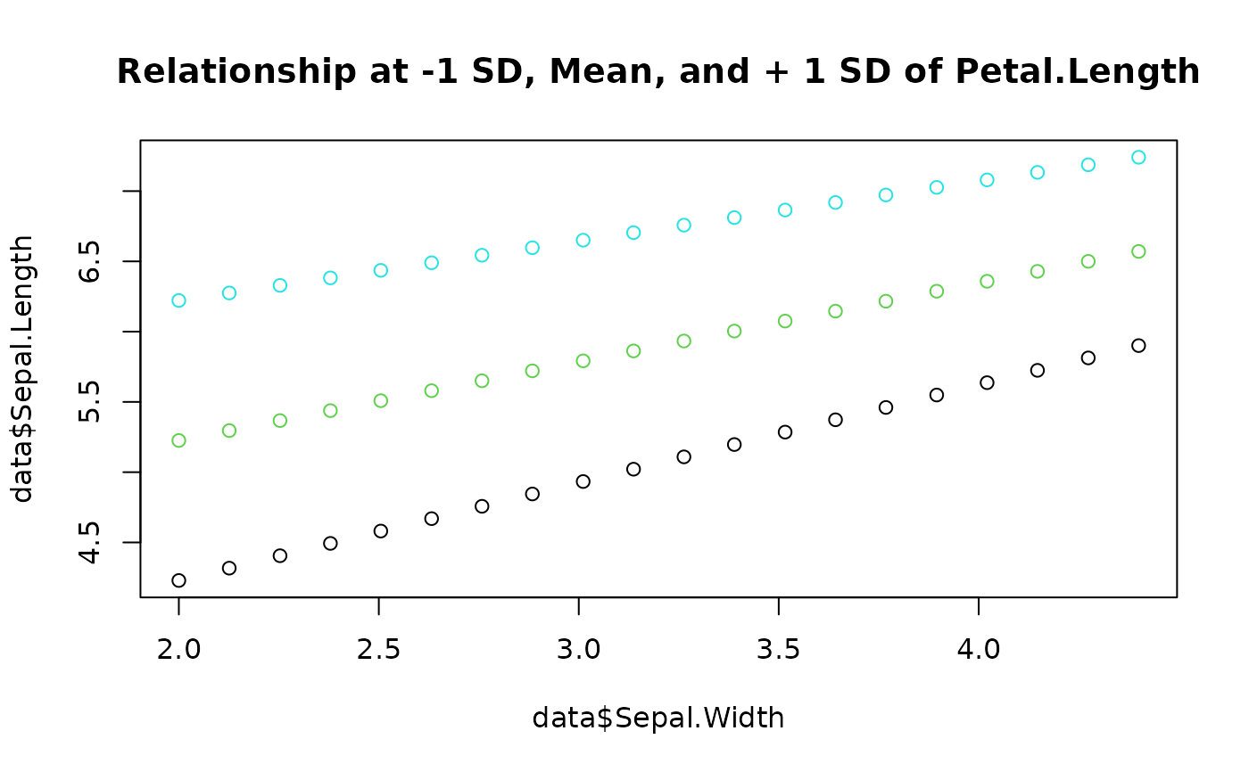
data <- get_datagrid(model, length = c(20, 3), range = c("range", "sd"))
# same as: get_datagrid(model, range = "grid", length = 20)

# Add predictions
data$Sepal.Length <- get_predicted(model, data = data)

# Visualize relationships (each color is at -1 SD, Mean, and + 1 SD of Petal.Length)
plot(data$Sepal.Width, data$Sepal.Length,
  col = data$Petal.Length,
  main = "Relationship at -1 SD, Mean, and + 1 SD of Petal.Length"
)

Usage

Arguments

Value

Details

See also

Examples