
Case Study: Intersectionality Analysis Using The MAIHDA Framework
Source:vignettes/practical_intersectionality.Rmd
practical_intersectionality.RmdThis vignette demonstrate how to use modelbased in the context of an intersectional multilevel analysis of individual heterogeneity, using the MAIHDA framework. The general approach of the MAIHDA framework (sometimes also I-MAIHDA) is described in Axelsson Fisk et al. (2018) and Evans et al. (2024).
Intersectionality analysis is a new approach in social epidemiology, which attempts to move away from looking at relevant social indicators in isolation.
“The advantage of incorporating an intersectional framework in social epidemiology is that it goes beyond the unidimensional study of socioeconomic and demographic categorizations by considering the effect of belonging to specific strata simultaneously defined by multiple social, economic and demographic dimensions.”
The steps we are showing here are:
Defining the intersectional strata.
Fitting a simple intersectional model to see whether intersectional strata contribute to between-stratum variance (which can be considered as “inequalities”, whether social or health related - also known as discriminatory accucarcy).
Fitting partially-adjusted intersectional models and calculating proportional change in the between-stratum variance (PCVs) to quantify to what degree the different intersectional dimensions contribute to the between-stratum variance (inequalities)
Fitting an intersectional interaction model to look for global additive or multiplicative effects.
Calculate adjusted / ranked predictions (estimated marginal means) of the outcome (of the simple intersectional model) by intersectional strata, to get a clearer picture of the variation between intersectional dimensions, as well as testing specific strata for significant differences.
Look at group-level estimates (BLUPs) of the intersectional interaction model, which represent the group-level residuals (also called strata-level residuals, see Axelsson Fisk et al. (2018) or Keller et al. (2023)), to see whether we find specific additive or multiplicative effects for strata.
1. Preparing the data and defining intersectional strata
First, we load the required packages and prepare a sample data set.
We use the efc data from the modelbased
package, which contains data of family carers who care for their elderly
relatives. Our outcome of interest is quality of life of family
carers (score ranging from 0 to 25 points), the different dimensions of
the intersectionality groups are gender (male/female),
employment status (currently employed yes/no) and age
(three groups: until 40, 41 to 64 and 65 or older). We assume that there
might be health-related inequalities, i.e. the quality of life differs
depending on the characteristics that define our intersectional
strata.
library(modelbased) # predictions and significance testing
library(insight) # extracting random effects variances
library(datawizard) # data wrangling and preparation
library(parameters) # model summaries
library(performance) # model fit indices, ICC
library(glmmTMB) # multilevel modelling

# sample data set
data(efc, package = "modelbased")

efc <- efc |>
  # numeric to factors, set labels as levels
  to_factor(select = c("c161sex", "c172code", "c175empl")) |>
  # recode age into three groups
  recode_values(
    select = "c160age",
    recode = list(`1` = "min:40", `2` = 41:64, `3` = "65:max")
  ) |>
  # rename variables
  data_rename(
    select = c("c161sex", "c160age", "quol_5", "c175empl"),
    replacement = c("gender", "age", "qol", "employed")
  ) |>
  # age into factor, set levels, and change labels for education
  data_modify(age = factor(age, labels = c("-40", "41-64", "65+")))
To include the intersectional strata variables gender,
employed and age in our mixed model, we will
define them as interacting random effects (excluding main effects of
interactions): (1 | gender:employed:age) (see also below).
The idea is to have truly unique combinations in our model, similar as
if we would create a factor variable with all combinations manually:
efc$strata <- ifelse(
  is.na(efc$employed) | is.na(efc$gender) | is.na(efc$age),
  NA_character_,
  paste0(efc$gender, ", ", efc$employed, ", ", efc$age)
)
efc$strata <- factor(efc$strata)
data_tabulate(efc$strata)
#> efc$strata <categorical>
#> # total N=908 valid N=900
#>
#> Value              |   N | Raw % | Valid % | Cumulative %
#> -------------------+-----+-------+---------+-------------
#> Female, no, -40    |  37 |  4.07 |    4.11 |         4.11
#> Female, no, 41-64  | 238 | 26.21 |   26.44 |        30.56
#> Female, no, 65+    | 135 | 14.87 |   15.00 |        45.56
#> Female, yes, -40   |  63 |  6.94 |    7.00 |        52.56
#> Female, yes, 41-64 | 210 | 23.13 |   23.33 |        75.89
#> Female, yes, 65+   |   3 |  0.33 |    0.33 |        76.22
#> Male, no, -40      |  15 |  1.65 |    1.67 |        77.89
#> Male, no, 41-64    |  42 |  4.63 |    4.67 |        82.56
#> Male, no, 65+      |  50 |  5.51 |    5.56 |        88.11
#> Male, yes, -40     |  34 |  3.74 |    3.78 |        91.89
#> Male, yes, 41-64   |  70 |  7.71 |    7.78 |        99.67
#> Male, yes, 65+     |   3 |  0.33 |    0.33 |       100.00
#> <NA>               |   8 |  0.88 |    <NA> |         <NA>
We now have the choice and could either use the strata
variable as group factor for our random effects, or
gender:employed:age. For plotting predictions (see section
4), we get clearer plots when we include the three factors
gender, employed and age instead
of the integrated strata factor.
2. Fitting the simple intersectional model: discriminatory accuracy
Intersectionality analysis aims at recognizing effects of belonging to specific strata simultaneously. In the context of the MAIHDA framework, the interest lies in analysing the variation between strata regarding the outcome of interest. Thus, the indicators that define the intersectional dimensions are used as interacting random effects (group factors) in a multilevel model (random-intercept model).
We start by fitting a linear mixed effects model, which includes no
fixed effects, but only our different intersectional dimensions:
gender, employed and age.
# Quality of Life score ranges from 0 to 25
m_null <- glmmTMB(qol ~ 1 + (1 | gender:employed:age), data = efc)

# the above model is identical to:
# m_null <- glmmTMB(qol ~ 1 + (1 | strata), data = efc)
The purpose of this model - which is sometimes also called null
model or base model - is to quantify the “discriminatory
accuracy”, which is achieved by calculating the ICC (see performance::icc())
of this model (sometimes also calles the VPC, the variance
partition coefficient). The higher the ICC, the greater the degree of
similarity within the strata (regarding quality of life) and
the greater the difference in quality of life between the
intersectional strata. I.e., the higher the ICC, the better the
model is at discriminating individuals with higher or lower quality of
life score, as opposed to models with lower ICC.
We now look at the model parameters and the ICC of our simple intersectional model.
model_parameters(m_null)
#> # Fixed Effects
#>
#> Parameter   | Coefficient |   SE |         95% CI |     z |      p
#> ------------------------------------------------------------------
#> (Intercept) |       14.91 | 0.40 | [14.13, 15.70] | 37.41 | < .001
#>
#> # Random Effects
#>
#> Parameter                           | Coefficient |       95% CI
#> ----------------------------------------------------------------
#> SD (Intercept: gender:employed:age) |        1.03 | [0.56, 1.89]
#> SD (Residual)                       |        5.23 | [4.99, 5.48]

icc(m_null)
#> # Intraclass Correlation Coefficient
#>
#>     Adjusted ICC: 0.038
#>   Unadjusted ICC: 0.038
The ICC with a value of about 4% is rather low. Usually, this indicates that our dimensions used to define the intersectional strata do not suggest larger social inequalities regarding quality of life. But we ignore this fact for now, as the purpose of demonstrating the analysis approach is rarely affected.
3. Partially-adjusted intersectional model and PCV
In the next step we want to find out, which intersectional dimension
contributes most to possible inequalities, i.e. which of our group
factors gender, employed and age
explains most of the between-stratum variance of the random effects.
This is achieved by fitting partially-adjusted intersectional
models.
“The purpose of the partially adjusted model was to quantify to what degree the different dimensions used to construct the intersectional strata contributed to the between stratum variance seen in the previous model.”
For each of the intersectional dimensions, a multilevel model including this dimension as fixed effect is fitted. We can then both look at the ICCs of the partially-adjusted models, as well as at the proportional change in the between-stratum variance, the so-called PCV coefficients.
First, we fit three models each with one dimension as predictor.
m_gender <- glmmTMB(qol ~ gender + (1 | gender:employed:age), data = efc)
m_employment <- glmmTMB(qol ~ employed + (1 | gender:employed:age), data = efc)
m_age <- glmmTMB(qol ~ age + (1 | gender:employed:age), data = efc)
The regression coefficients already give an impression how strong the association between each single dimension and the outcome is, taking between-stratum variance into account. The larger (in absolute values) the coefficients, the higher the degree that dimension contributed to the between-stratum variance.
compare_parameters(m_gender, m_employment, m_age)
#> Parameter       |             m_gender |         m_employment |                m_age
#> ------------------------------------------------------------------------------------
#> (Intercept)     | 15.55 (14.51, 16.60) | 14.23 (13.35, 15.12) | 16.25 (15.33, 17.17)
#> gender [Female] | -1.18 (-2.54,  0.17) |                      |
#> employed [yes]  |                      |  1.38 ( 0.07,  2.68) |
#> age [41-64]     |                      |                      | -1.99 (-3.14, -0.84)
#> age [65+]       |                      |                      | -2.55 (-3.88, -1.23)
#> ------------------------------------------------------------------------------------
#> Observations    |                  895 |                  895 |                  895
Looking at the summary tables above, it seems like
gender is the dimension that explains least of the
between-stratum variance, i.e. gender seems to be the characteristic
that contributes least to potential social inequalities.
age, in turn, seems to be the most important characteristic
regarding inequalities.
Since the fixed effects now take away some of the proportion of the variance explained by the grouping factors (random effects), we expect the ICC for the above models to be lower.
icc(m_gender)$ICC_adjusted
#> [1] 0.02583979
icc(m_employment)$ICC_adjusted
#> [1] 0.02341412
icc(m_age)$ICC_adjusted
#> [1] 0.00461901
Indeed, the ICC correlates with the fixed effects coefficients, i.e. the larger the coefficient (in absolute values), the lower the ICC.
Next, we want to quantify the degree the different dimensions contribute to the variance between groups more accurately. To do so, we calculate the proportional change in between-stratum variance, or PCV. This coefficient explains how much of the total proportion of explained variance by the strata can be explained by a single dimension that define those strata. The PCV ranges from 0 to 1, and the closer to 1, the more this particular dimension explains social inequalities.
# extract random effect variances from all models
v_null <- get_variance(m_null)
v_gender <- get_variance(m_gender)
v_employment <- get_variance(m_employment)
v_age <- get_variance(m_age)

# PCV (proportional change in between-stratum variance)
# from null-model to gender-model
(v_null$var.random - v_gender$var.random) / v_null$var.random
#> [1] 0.3202535

# PCV from null-model to employment-model
(v_null$var.random - v_employment$var.random) / v_null$var.random
#> [1] 0.3859538

# PCV from null-model to age-model
(v_null$var.random - v_age$var.random) / v_null$var.random
#> [1] 0.8809532
Again, we see that the PCV is in line with the models’ ICC’s and
regression coefficients. We see the highest proportional change for
age, meaning that - although gender and education can
contribute to inequalities - age is the most relevant predictor.
4. PCV in the intersectional interaction model: global additive or multiplicative effects
Finally, a “full” model (aka intersectional interaction or main effects model) is fit, which includes all group level variables as level-1 additive fixed effects. Then, the PCV is again calculated. This allows us to see how much of the variability of the additive effects will be absorbed by the intersectional strata characteristics. A PCV close to 1 suggests that the differences between intersectional strata are primarily driven by additive main effects. Conversely, a PCV substantially below 1 indicates that these main effects cannot fully explain the strata-level variance, pointing to the presence of multiplicative interaction effects.
m_full <- glmmTMB(
  qol ~ gender + employed + age + (1 | gender:employed:age),
  data = efc
)

# investigate random effects parameters
random_parameters(m_full)
#> # Random Effects
#>
#> Within-Group Variance                     27.1 (5.21)
#> Between-Group Variance
#>   Random Intercept (gender:employed:age)     0    (0)
#> N (groups per factor)
#>   gender                                     2
#>   employed                                   2
#>   age                                        3
#> Observations                               895
We see that the between-group variance is literally zero, which means, no variation is left between the intersectional strata after adding those predictors as additive fixed effects. This suggests that the PCV will be (close to) 1, indicating we have no multiplicative interaction effects.
v_full <- get_variance(m_full)

# PCV (proportional change in between-stratum variance)
# from null-model to full-model
(v_null$var.random - v_full$var.random) / v_null$var.random
#> [1] 1
Indeed, the PCV for the full model is 1.
The ICC (or VPC) and the PCV are global measures of intersectionality (“are there differences between intersectional strata” and “are there additive or multiplicative effects and which characteristic contributes most to inequalities?”). There is also an additional specific measure of intersectionality (“which intersections may show multiplicative effects?”), the strata-level residuals, which will be introduced below.
5. Predict between-stratum variance and test for significant differences
Finally, we may want to have a clearer picture of how the different strata vary, which combination of characteristics defines the highest or maybe lowest risk group. To do so, we calculate predictions of the random effects (unit-level predictions).
The following code shows the predicted average quality of life scores for the different groups.
predictions <- estimate_means(
  m_null,
  by = c("gender", "employed", "age"),
  estimate = "average"
)
plot(predictions)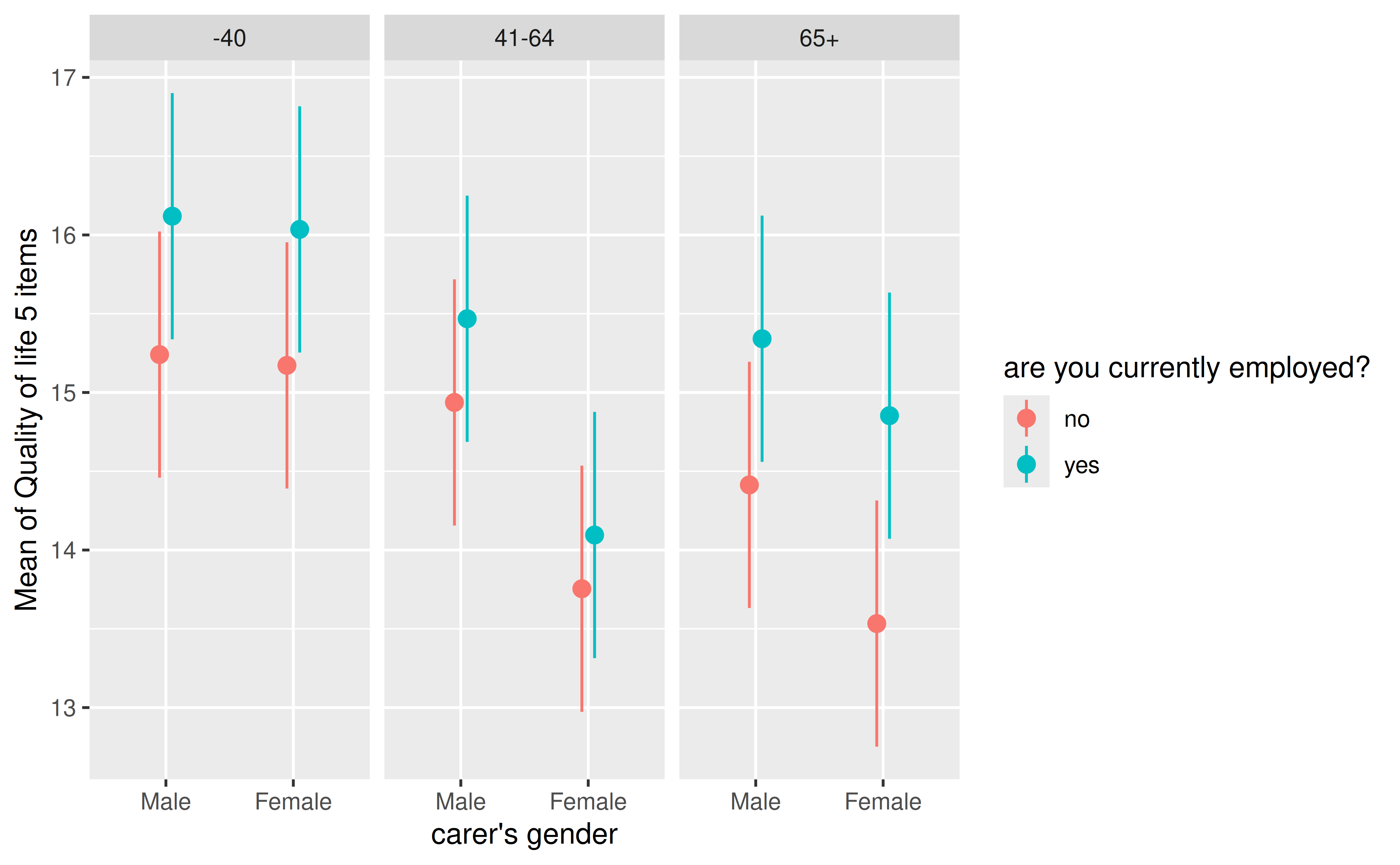
According to these results, employed male family carers, who are not older than 40 years, show on average the highest quality of life. On the other hand, unemployed female carers aged 65 or older have the lowest quality of life.
We can now calculate pairwise comparisons that show which differences between groups are statistically significant. Since all combinations of pairwise comparisons would return 66 rows in total, we just show the first ten rows for demonstrating purpose.
# just show first 10 rows of output...
estimate_contrasts(
  m_null,
  contrast = c("gender", "employed", "age"),
  estimate = "average"
)[1:10, ]
#> Averaged Contrasts Analysis
#>
#> Level1             | Level2        | Difference (CI)
#> ----------------------------------------------------
#> Male, no, 41-64    | Male, no, -40 |           -0.30
#> Male, no, 65++     | Male, no, -40 |           -0.83
#> Male, yes, -40     | Male, no, -40 |            0.88
#> Male, yes, 41-64   | Male, no, -40 |            0.23
#> Male, yes, 65++    | Male, no, -40 |            0.10
#> Female, no, -40    | Male, no, -40 |           -0.07
#> Female, no, 41-64  | Male, no, -40 |           -1.49
#> Female, no, 65++   | Male, no, -40 |           -1.71
#> Female, yes, -40   | Male, no, -40 |            0.79
#> Female, yes, 41-64 | Male, no, -40 |           -1.15
#>
#> Variable predicted: qol
#> Predictors contrasted: gender, employed, age
#> p-values are uncorrected.
If we only want to modulate one factor and compare those groups
within the levels of the other groups, we can use the by
argument. This reduces the output and only compares the focal term(s)
within the levels of the remaining predictors.
# Compare levels of gender and employment status for age groups
estimate_contrasts(
  m_null,
  contrast = c("gender", "employed"),
  by = "age",
  estimate = "average"
)
#> Averaged Contrasts Analysis
#>
#> Level1      | Level2     | Difference (CI) |   age
#> --------------------------------------------------
#> Male, yes   | Male, no   | 0.88            |   -40
#> Female, no  | Male, no   | -0.07           |   -40
#> Female, yes | Male, no   | 0.79            |   -40
#> Female, no  | Male, yes  | -0.95           |   -40
#> Female, yes | Male, yes  | -0.08           |   -40
#> Female, yes | Female, no | 0.86            |   -40
#> Male, yes   | Male, no   | 0.53            | 41-64
#> Female, no  | Male, no   | -1.18           | 41-64
#> Female, yes | Male, no   | -0.84           | 41-64
#> Female, no  | Male, yes  | -1.71           | 41-64
#> Female, yes | Male, yes  | -1.37           | 41-64
#> Female, yes | Female, no | 0.34            | 41-64
#> Male, yes   | Male, no   | 0.93            |   65+
#> Female, no  | Male, no   | -0.88           |   65+
#> Female, yes | Male, no   | 0.44            |   65+
#> Female, no  | Male, yes  | -1.81           |   65+
#> Female, yes | Male, yes  | -0.49           |   65+
#> Female, yes | Female, no | 1.32            |   65+
#>
#> Variable predicted: qol
#> Predictors contrasted: gender, employed
#> p-values are uncorrected.
E.g., if we look at the plot and want to know whether female persons aged 65+ differ depending on their employment status, we can use the following code:
# Compare levels employment status by gender and age groups
estimate_contrasts(
  m_null,
  contrast = "employed",
  by = c("gender", "age"),
  estimate = "average"
)
#> Averaged Contrasts Analysis
#>
#> Level1 | Level2 | Difference (CI) | gender |   age
#> --------------------------------------------------
#> yes    | no     | 0.88            | Male   |   -40
#> yes    | no     | 0.86            | Female |   -40
#> yes    | no     | 0.53            | Male   | 41-64
#> yes    | no     | 0.34            | Female | 41-64
#> yes    | no     | 0.93            | Male   |   65+
#> yes    | no     | 1.32            | Female |   65+
#>
#> Variable predicted: qol
#> Predictors contrasted: employed
#> p-values are uncorrected.
6. Strata-level residuals: Specific additive vs. multiplicative effects
In the MAIHDA framework, a specific measure of intersectionality is the strata-level residual, which corresponds to the random effects of the intersectional interaction model. Examining these residuals allows us to distinguish between additive and multiplicative effects: if there are no interactions, the inclusion of main effects would fully explain the variance between intersectional strata and all random effects would be (close to) zero. A positive strata-level residual indicates that a stratum’s mean outcome is higher than expected from the additive main effects, whereas a negative strata-level residual indicates a lower mean outcome than expected for this stratum. Consequently, when the credible or confidence interval of a strata-level residual does not include zero, this points to a statistically significant interaction effect – or a multiplicative effect – in that specific stratum (Axelsson Fisk et al. 2018; Keller et al. 2023).
We can easily compute the strata-level residuals using the
estimate_grouplevel() function. Important:
We need to calculate these residuals for the intersectional
interaction (full) model, not for the null model.
strata_residuals <- estimate_grouplevel(m_full)

strata_residuals
#> Group               | Level            | Parameter   | Coefficient |       SE |        95% CI
#> ---------------------------------------------------------------------------------------------
#> gender:employed:age | Female:no:-40    | (Intercept) |   -2.23e-09 | 1.46e-04 | [ 0.00, 0.00]
#> gender:employed:age | Female:no:41-64  | (Intercept) |    1.58e-08 | 1.49e-04 | [ 0.00, 0.00]
#> gender:employed:age | Female:no:65+    | (Intercept) |    1.80e-09 | 1.46e-04 | [ 0.00, 0.00]
#> gender:employed:age | Female:yes:-40   | (Intercept) |    1.95e-08 | 1.50e-04 | [ 0.00, 0.00]
#> gender:employed:age | Female:yes:41-64 | (Intercept) |   -3.58e-08 | 1.60e-04 | [ 0.00, 0.00]
#> gender:employed:age | Female:yes:65+   | (Intercept) |    9.71e-10 | 1.46e-04 | [ 0.00, 0.00]
#> gender:employed:age | Male:no:-40      | (Intercept) |   -9.86e-09 | 1.47e-04 | [ 0.00, 0.00]
#> gender:employed:age | Male:no:41-64    | (Intercept) |    6.36e-09 | 1.46e-04 | [ 0.00, 0.00]
#> gender:employed:age | Male:no:65+      | (Intercept) |   -1.19e-08 | 1.47e-04 | [ 0.00, 0.00]
#> gender:employed:age | Male:yes:-40     | (Intercept) |   -7.41e-09 | 1.46e-04 | [ 0.00, 0.00]
#> gender:employed:age | Male:yes:41-64   | (Intercept) |    1.37e-08 | 1.48e-04 | [ 0.00, 0.00]
#> gender:employed:age | Male:yes:65+     | (Intercept) |    9.11e-09 | 1.47e-04 | [ 0.00, 0.00]

plot(strata_residuals)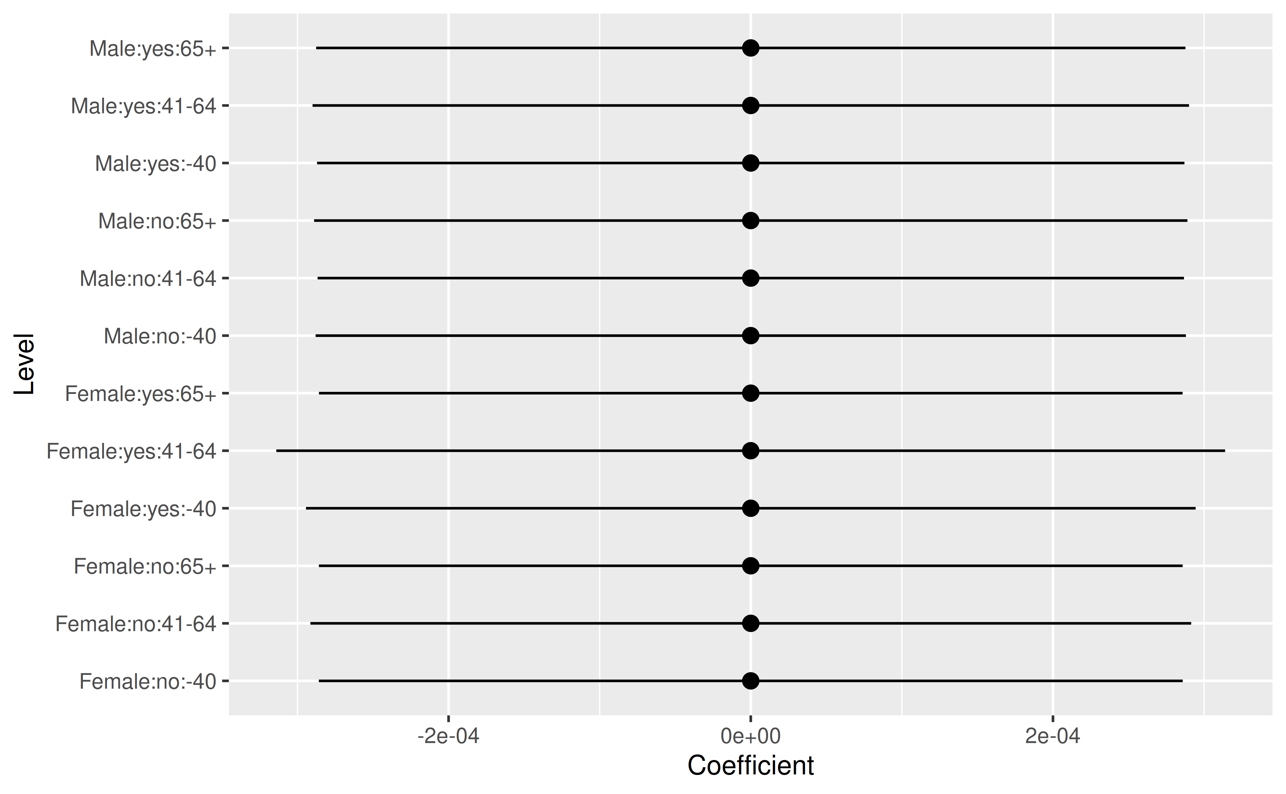
As expected (because the PCV is 1, indicating we found no multiplicative effects), all strata-level residuals are close to zero.
7. MAIHDA and logistic regression models
Compared to a MAIHDA analysis using linear regression models, there are two important aspects to consider when using binary logistic regression models.
7.1 Additive and multiplicatice effects
When applying this framework to dichotomous outcomes using logistic
multilevel models, two important distinctions must be considered. First,
the within-strata (level 1) variance is not estimated, as the variance
of the binomial distribution is already known (and fixed, see ?insight::get_variance
for Bernoulli models). Second, logistic models operate on a
multiplicative scale rather than an additive one. According to Evans et
al. (2018), it is inappropriate to use logistic models to examine
strata-level residuals for additive interaction effects, since the
inclusion of main effects may already account for some of these
interactions. However, logistic models remain fully appropriate if the
primary goal is to estimate strata-level effects to explore the overall
patterning of inequalities across strata-groups (Evans et al. 2018).
7.2 Discriminatory Accuracy
In the case of linear models, the ICC (VPC) works as measure of discriminatory accuracy. However, since the ICC relies on the estimated variances on level-1 and the higher levels and the level-1 variance is not estimable in logistic regression models, we need a different measure for the discriminatory accuracy.
In the context of logistic regression for dichotomous
outcomes, the Area Under the Curve (AUC) serves as a measure of
discriminatory accuracy (which can be calculated using performance::performance_roc()
or performance::performance_accuracy()).
It evaluates how accurately knowing an individual’s intersectional
stratum can discriminate between those who experience the outcome and
those who do not. Formally, the AUC represents the probability that a
randomly selected individual with the outcome will have a higher
predicted probability than a randomly selected individual without it.
The AUC ranges from 0.5 to 1.0 (or 50% to 100%), where 0.5 indicates
that the intersectional strata provide no discriminatory accuracy, and
1.0 denotes perfect discriminatory accuracy (Evans et al. 2024).
Another useful measure is the median odds ratio (MOR), a measure of cluster-level variation in multilevel logistic regression (Larsen and Merlo 2005). A MOR > 1 indicates the presence of heterogeneity and meaningful variation across clusters.
8. Conclusion
Intersectional multilevel analysis of individual heterogeneity, using the MAIHDA framework, is a new approach in social epidemiology, which helps to understand the interaction of social indicators with regard to social inequalities.
This approach requires the application of multilevel models, where ICC and PCV are relevant coefficients. The modelbased package allows to go beyond quantifying to what degree different intersectional dimensions contribute to inequalities by predicting the average outcome by group, thereby explicitly showing the differences between those groups (strata).
Furthermore, with modelbased it is possible to compare differences between groups and test whether these differences are statistically significant or not, i.e. whether we find “evidence” for social inequalities in our data for certain groups (at risk).