Sometimes, for instance for visualization purposes, we want to extract a reference grid (or data grid) of our dataset, that we will call a visualisation matrix. This reference grid usually contains the same variables than the original dataset, but reorganized in a particular, balanced, way. For instance, it might contain all the combinations of factors, or equally spread points of a continuous variable. These reference grids are often used as data for predictions of statistical models, to help us represent and understand them.
Simple linear regression
For instance, let’s fit a simple linear model that models the
relationship between Sepal.Width and
Sepal.Length.
library(easystats)
library(ggplot2)

model <- lm(Sepal.Width ~ Sepal.Length, data = iris)
parameters(model)
> Parameter | Coefficient | SE | 95% CI | t(148) | p
> -------------------------------------------------------------------
> (Intercept) | 3.42 | 0.25 | [ 2.92, 3.92] | 13.48 | < .001
> Sepal Length | -0.06 | 0.04 | [-0.15, 0.02] | -1.44 | 0.152The most obvious way of representing this model is to plot the data
points and add the regression line using the geom_smooth
function from ggplot2:
ggplot(iris, aes(x = Sepal.Length, y = Sepal.Width)) +
  geom_point() +
  geom_smooth(method = "lm") +
  theme_minimal()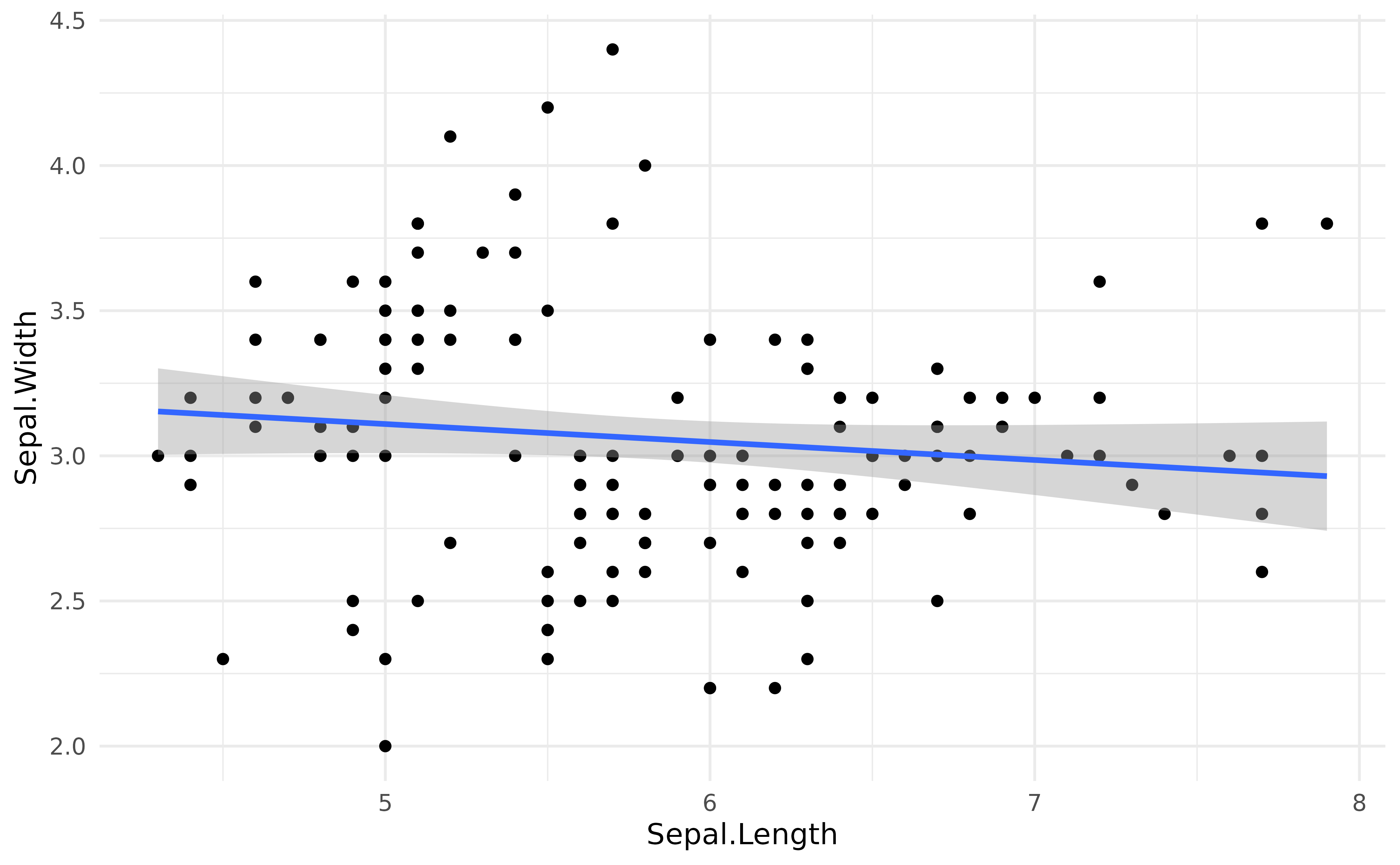
But how to “access” the data of this regression line? One good option
is to select some values of of the predictor
(Sepal.Length), and predict (using the
base R predict() method for now) the response
(Sepal.Width) using the model. Using these x and
y points, we can then create the regression line.
Let’s try the get_datagrid()
function from the insight package.
get_datagrid(iris["Sepal.Length"])> Visualisation Grid
>
> Sepal.Length
> ------------
> 4.30
> 4.70
> 5.10
> 5.50
> 5.90
> 6.30
> 6.70
> 7.10
> 7.50
> 7.90If we pass a numeric column to the function, it will return a vector
of equally spread points (having the same range, i.e.,
the same minimum and maximum, than the original data). The default
length is 10, but we can adjust that through the
length argument. For instance, for linear relationships
(i.e., a straight line), two points are in theory sufficient. Let’s
generate predictions using this reference grid of the predictor.
vizdata <- get_datagrid(iris["Sepal.Length"], length = 2)
vizdata$Predicted <- predict(model, vizdata)
vizdata
> Visualisation Grid
>
> Sepal.Length | Predicted
> ------------------------
> 4.30 | 3.15
> 7.90 | 2.93Now that we have our x and y values, we can plot the line as an overlay to the actual data points:
ggplot(iris, aes(x = Sepal.Length, y = Sepal.Width)) +
  geom_point() +
  geom_line(data = vizdata, aes(y = Predicted), linewidth = 1, color = "red") +
  theme_minimal()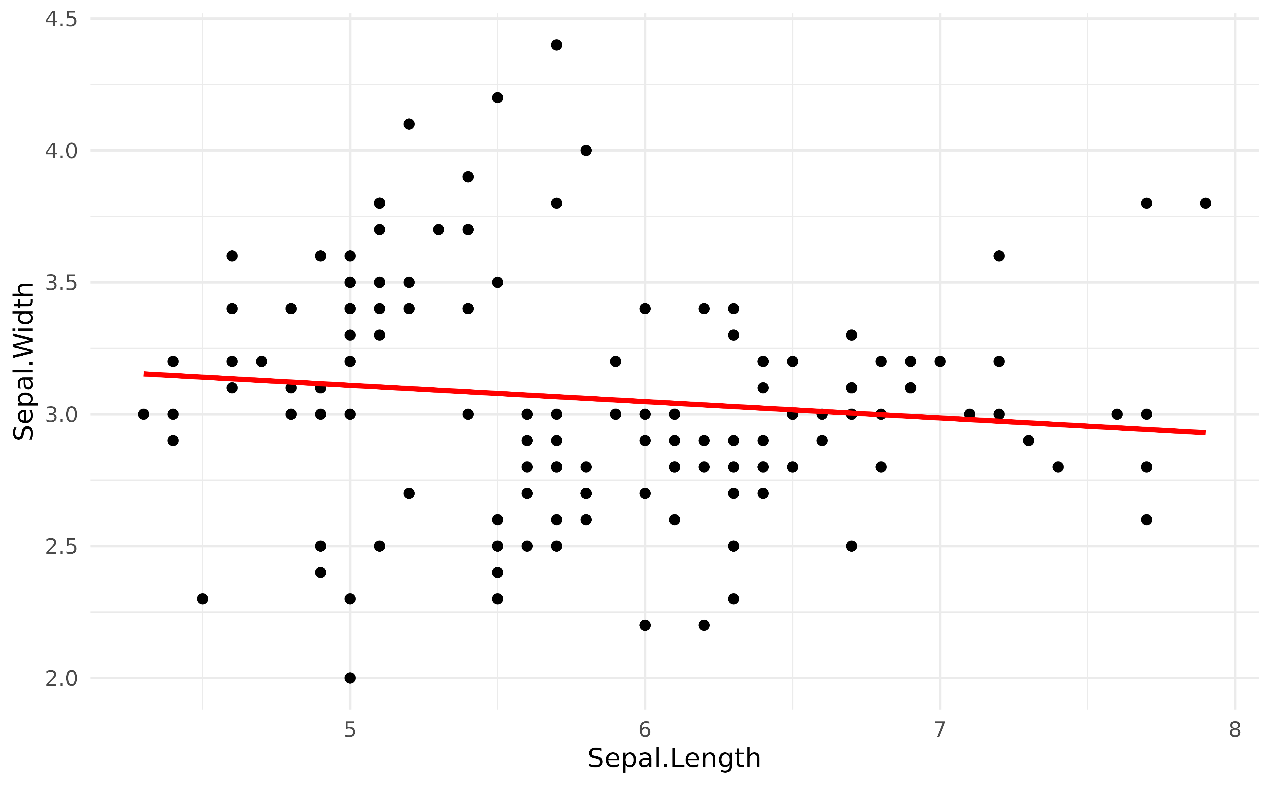
As we can see, it is quite similar to the previous plot. So, when can this be useful?
Mixed models
Data grids are useful to represent more complex models. For instance, in the models above, the negative relationship between the length and width of the sepals is in fact biased by the presence of three different species. One way of adjusting the model for this grouping structure is to add it as a random effect in a mixed model. In the model below, the “fixed” effects (the parameters of interest) will be adjusted (“averaged over”) to the random effects.
library(lme4)

model <- lmer(Sepal.Width ~ Sepal.Length + (1 | Species), data = iris)
parameters(model)
> # Fixed Effects
>
> Parameter | Coefficient | SE | 95% CI | t(146) | p
> ------------------------------------------------------------------
> (Intercept) | 1.04 | 0.43 | [0.20, 1.89] | 2.45 | 0.015
> Sepal Length | 0.34 | 0.05 | [0.25, 0.44] | 7.47 | < .001
>
> # Random Effects
>
> Parameter | Coefficient
> -------------------------------------
> SD (Intercept: Species) | 0.57
> SD (Residual) | 0.29As we can see, when adjusting for the species, the relationship between the two variables has become positive!
We can represent it using the same procedure as above, but note that
instead of using the base R predict() function, we will be
using get_predicted(),
from the insight package, which is a more robust and
user-friendly version of predict().
vizdata <- get_datagrid(iris["Sepal.Length"])
vizdata$Predicted <- get_predicted(model, vizdata)

ggplot(iris, aes(x = Sepal.Length, y = Sepal.Width)) +
  geom_point(aes(color = Species)) +
  geom_line(data = vizdata, aes(y = Predicted), linewidth = 1) +
  theme_minimal()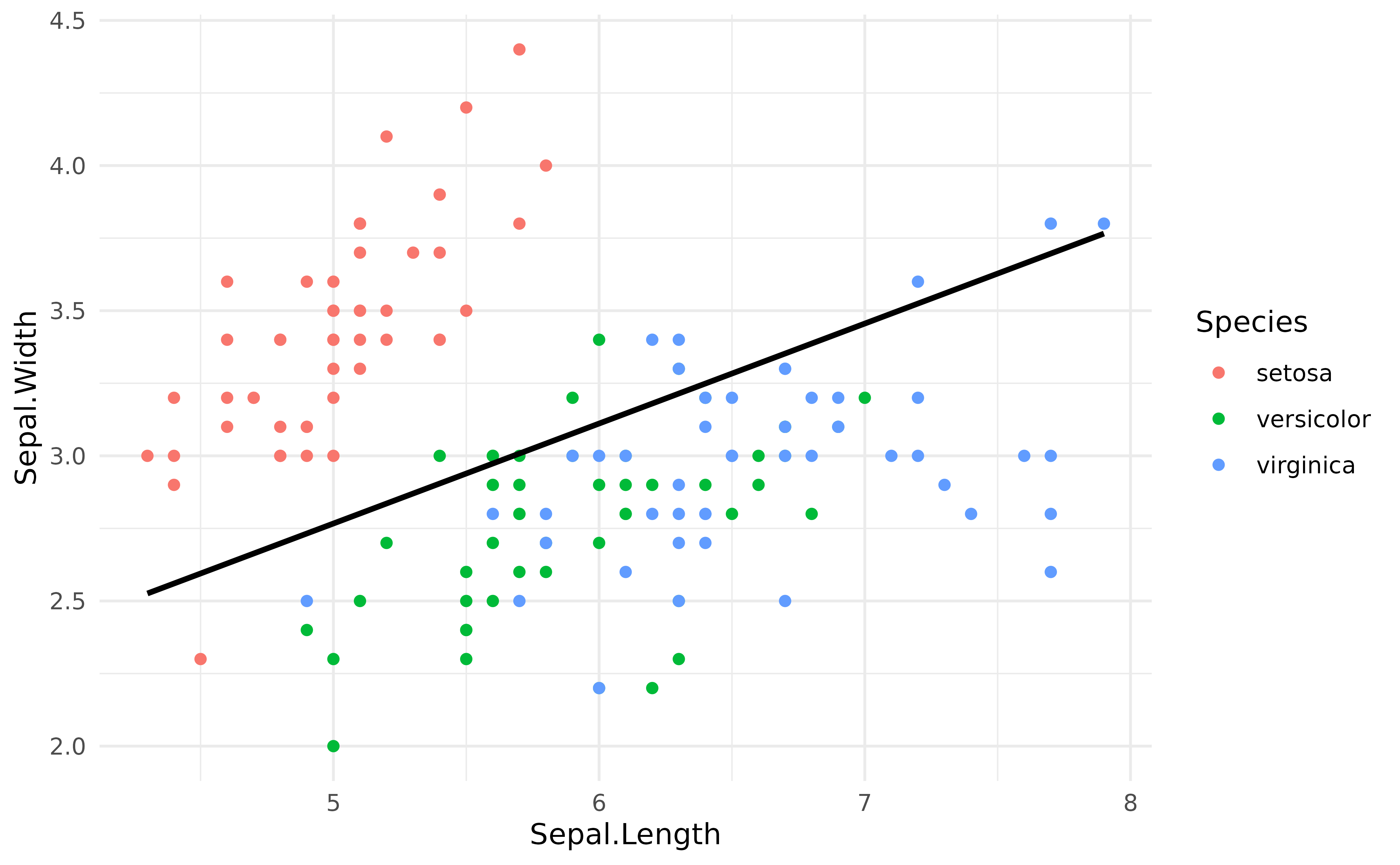
Fixed variables
The above way of constructing the reference grid, i.e., by providing a single column of data to the function, is almost equivalent to the following:
vizdata <- get_datagrid(iris, by = "Sepal.Length")
vizdata
> Visualisation Grid
>
> Sepal.Length | Sepal.Width | Petal.Length | Petal.Width | Species
> -----------------------------------------------------------------
> 4.30 | 3.06 | 3.76 | 1.20 | setosa
> 4.70 | 3.06 | 3.76 | 1.20 | setosa
> 5.10 | 3.06 | 3.76 | 1.20 | setosa
> 5.50 | 3.06 | 3.76 | 1.20 | setosa
> 5.90 | 3.06 | 3.76 | 1.20 | setosa
> 6.30 | 3.06 | 3.76 | 1.20 | setosa
> 6.70 | 3.06 | 3.76 | 1.20 | setosa
> 7.10 | 3.06 | 3.76 | 1.20 | setosa
> 7.50 | 3.06 | 3.76 | 1.20 | setosa
> 7.90 | 3.06 | 3.76 | 1.20 | setosa
>
> Maintained constant: Sepal.Width, Petal.Length, Petal.Width, SpeciesHowever, the other variables (present in the dataframe but not
selected as at) are “fixed”, i.e., they are
maintained at specific values. This is useful when we have other
variables in the model in whose effect we are not interested.
By default, factors are fixed by their “reference” level and numeric variables are fixed at their mean. However, this can be easily changed:
vizdata <- get_datagrid(iris, by = "Sepal.Length", numerics = "min")
vizdata
> Visualisation Grid
>
> Sepal.Length | Sepal.Width | Petal.Length | Petal.Width | Species
> -----------------------------------------------------------------
> 4.30 | 2 | 1 | 0.10 | setosa
> 4.70 | 2 | 1 | 0.10 | setosa
> 5.10 | 2 | 1 | 0.10 | setosa
> 5.50 | 2 | 1 | 0.10 | setosa
> 5.90 | 2 | 1 | 0.10 | setosa
> 6.30 | 2 | 1 | 0.10 | setosa
> 6.70 | 2 | 1 | 0.10 | setosa
> 7.10 | 2 | 1 | 0.10 | setosa
> 7.50 | 2 | 1 | 0.10 | setosa
> 7.90 | 2 | 1 | 0.10 | setosa
>
> Maintained constant: Sepal.Width, Petal.Length, Petal.Width, SpeciesTarget variables
If more than one target variable is selected,
get_datagrid() will return the combination
of them (i.e., all unique values crossed together). This can be
useful in the case of an interaction between a numeric
variable and a factor.
Let’s visualise the regression line for each of the levels of
Species:
model <- lm(Sepal.Width ~ Sepal.Length * Species, data = iris)

vizdata <- get_datagrid(iris, by = c("Sepal.Length", "Species"), length = 5)
vizdata$Predicted <- get_predicted(model, vizdata)
vizdata
> Visualisation Grid
>
> Sepal.Length | Species | Sepal.Width | Petal.Length | Petal.Width | Predicted
> --------------------------------------------------------------------------------
> 4.30 | setosa | 3.06 | 3.76 | 1.20 | 2.86
> 5.20 | setosa | 3.06 | 3.76 | 1.20 | 3.58
> 6.10 | setosa | 3.06 | 3.76 | 1.20 | 4.30
> 7.00 | setosa | 3.06 | 3.76 | 1.20 | 5.02
> 7.90 | setosa | 3.06 | 3.76 | 1.20 | 5.74
> 4.30 | versicolor | 3.06 | 3.76 | 1.20 | 2.25
> 5.20 | versicolor | 3.06 | 3.76 | 1.20 | 2.53
> 6.10 | versicolor | 3.06 | 3.76 | 1.20 | 2.82
> 7.00 | versicolor | 3.06 | 3.76 | 1.20 | 3.11
> 7.90 | versicolor | 3.06 | 3.76 | 1.20 | 3.40
> 4.30 | virginica | 3.06 | 3.76 | 1.20 | 2.44
> 5.20 | virginica | 3.06 | 3.76 | 1.20 | 2.65
> 6.10 | virginica | 3.06 | 3.76 | 1.20 | 2.86
> 7.00 | virginica | 3.06 | 3.76 | 1.20 | 3.07
> 7.90 | virginica | 3.06 | 3.76 | 1.20 | 3.28
>
> Maintained constant: Sepal.Width, Petal.Length, Petal.Width
ggplot(iris, aes(x = Sepal.Length, y = Sepal.Width, color = Species)) +
  geom_point() +
  geom_line(data = vizdata, aes(y = Predicted), linewidth = 1) +
  theme_minimal()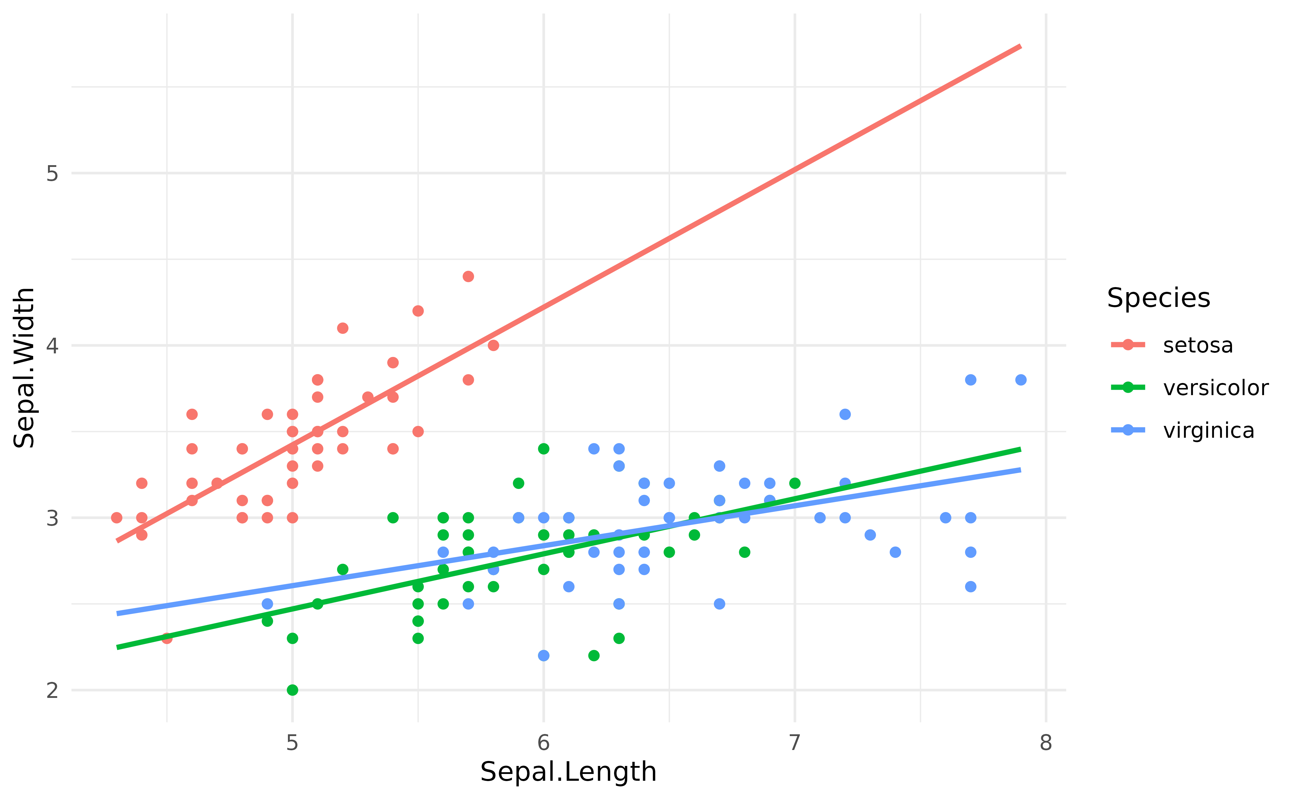
Preserve range
However, it is generally not a good practice to extend the regression
lines beyond the range of its original data, as it is the case here for
the red line. The preserve_range option
allows to remove observations that are “outside” the original dataset
(however, the length should be increased to improve the precision toward
the edges):
vizdata <- get_datagrid(iris,
  by = c("Sepal.Length", "Species"),
  length = 100,
  preserve_range = TRUE
)

vizdata$Predicted_Sepal.Width <- get_predicted(model, vizdata)

ggplot(iris, aes(x = Sepal.Length, y = Sepal.Width, color = Species)) +
  geom_point() +
  geom_line(data = vizdata, aes(y = Predicted_Sepal.Width), linewidth = 1) +
  theme_minimal()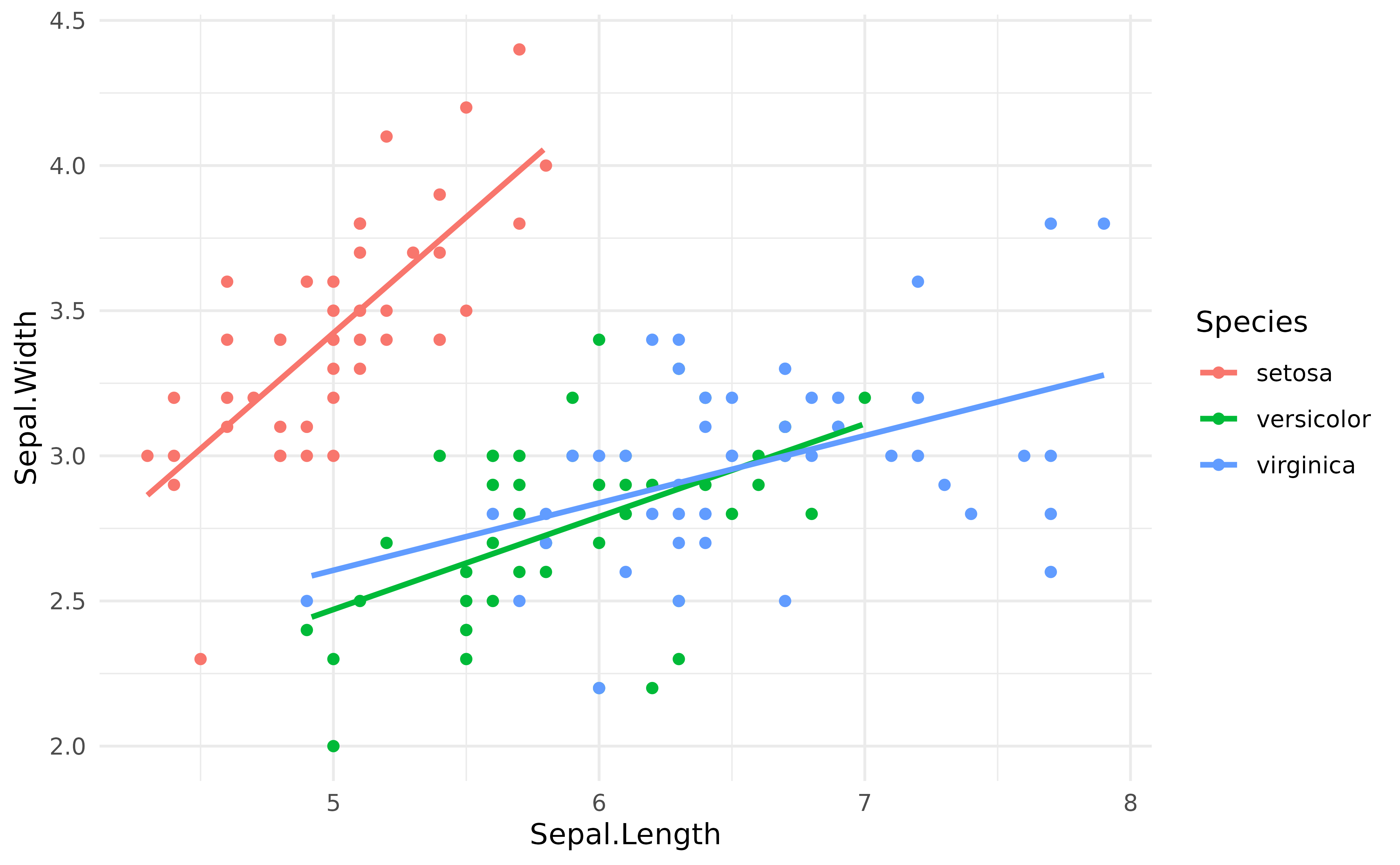
Visualising an interaction between two numeric variables (three-way interaction)
model <- lm(Sepal.Length ~ Petal.Length * Petal.Width, data = iris)
parameters(model)
> Parameter | Coefficient | SE | 95% CI | t(146) | p
> ----------------------------------------------------------------------------------
> (Intercept) | 4.58 | 0.11 | [ 4.36, 4.80] | 40.89 | < .001
> Petal Length | 0.44 | 0.07 | [ 0.31, 0.57] | 6.74 | < .001
> Petal Width | -1.24 | 0.22 | [-1.67, -0.81] | -5.65 | < .001
> Petal Length × Petal Width | 0.19 | 0.03 | [ 0.12, 0.25] | 5.62 | < .001This idea can also be used to visualise interactions between two numeric variables, aka the nightmare of every scientist. One possibility is to basically represent the relationship between the response and one predictor at a few representative values of the second predictor.
In this case, we will represent the regression line between
Sepal.Length and Petal.Length and a 5 equally
spaced values of Petal.Length, to get a feel for the
interaction.
We can obtain the right reference grid quite easily by chaining two data grids together as follows:
vizdata <- iris |>
  get_datagrid(c("Petal.Length", "Petal.Width"), length = 10) |>
  get_datagrid("Petal.Width", length = 5, numerics = "all")
What did we do here? We started by generating a reference grid
containing all the combinations between the 10 equally spread values of
the two target variables, creating 10 * 10 = 100 rows. The
next step was to reduce Petal.Length to a set of 5 values,
but without touching the other variables (i.e., keeping the 10
values created for Petal.Length). This was achieved using
numerics = "all".
We can then visualise it as follows:
vizdata$Predicted <- get_predicted(model, vizdata)

iris |>
  ggplot(aes(x = Petal.Length, y = Sepal.Length, color = Petal.Width)) +
  geom_point() +
  geom_line(data = vizdata, aes(y = Predicted, group = Petal.Width), linewidth = 1) +
  scale_color_viridis_c() +
  theme_minimal()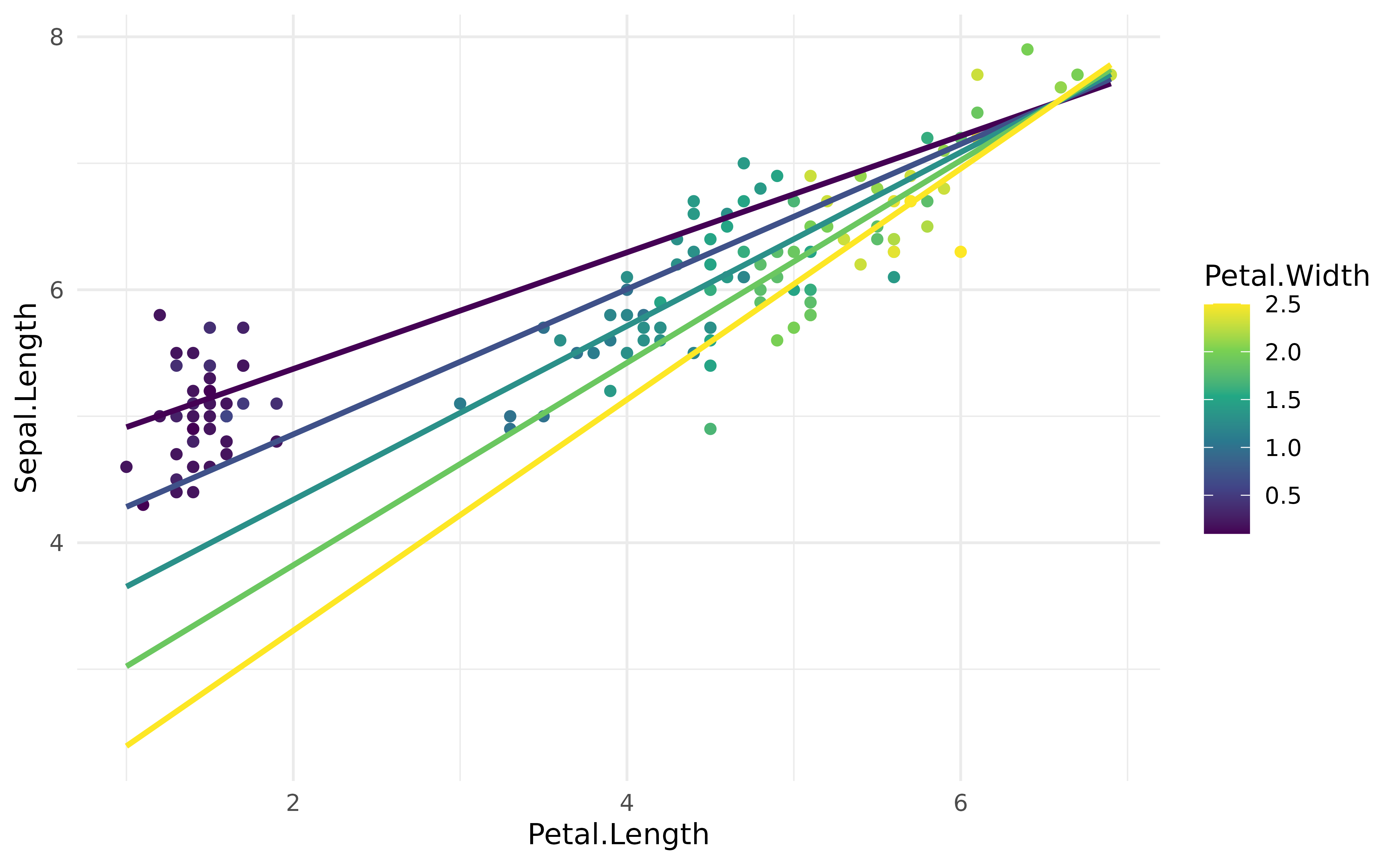
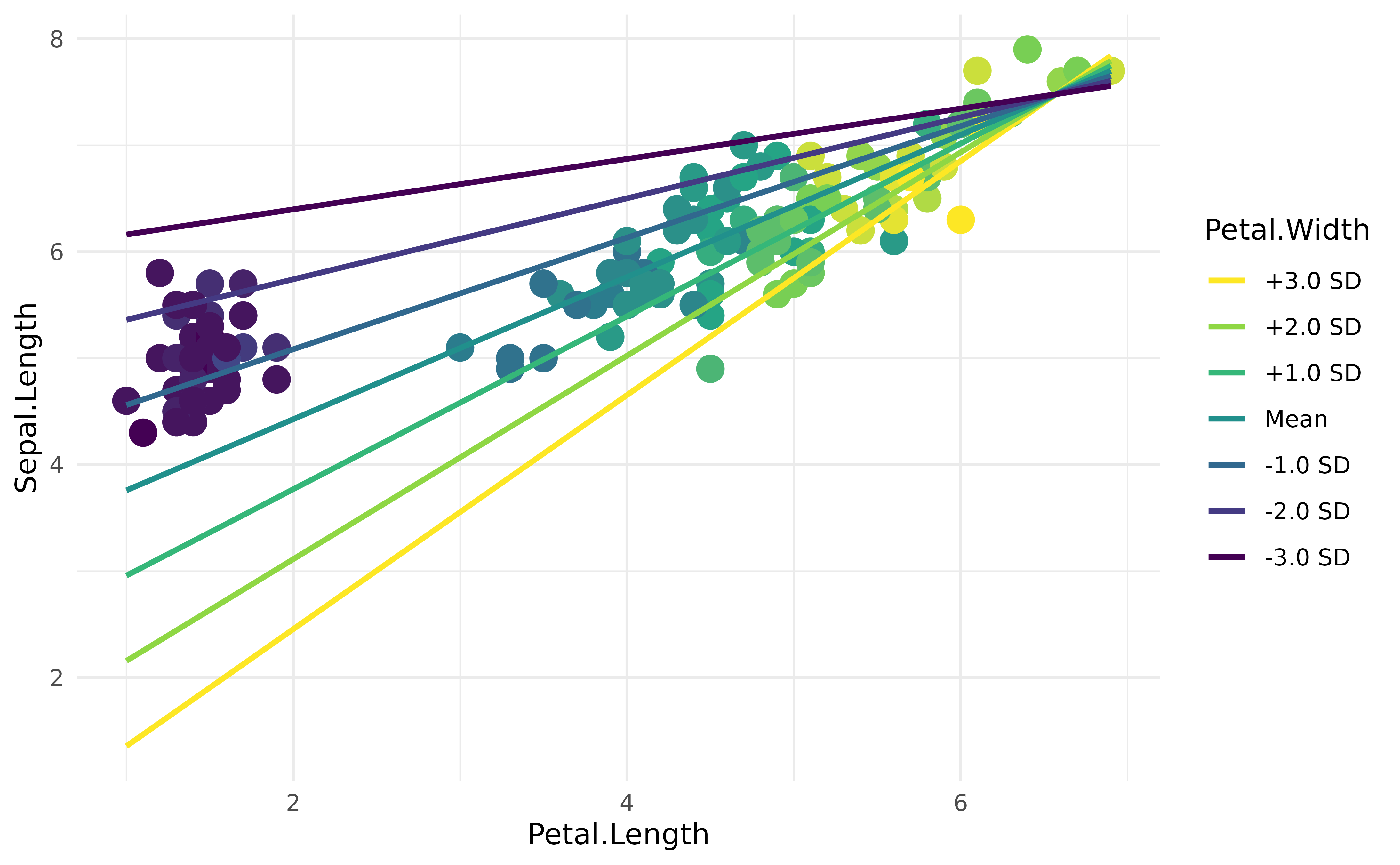
Such plot can be more clear by expressing the interaction variable in terms of deviations from the mean (as a standardized variable).
# Express values in an abstract way
vizdata$Petal.Width <- effectsize::format_standardize(
  vizdata$Petal.Width,
  reference = iris$Petal.Width
)

ggplot(iris, aes(x = Petal.Length, y = Sepal.Length)) +
  # Only shapes from 21 to 25 have a fill aesthetic
  geom_point2(aes(fill = Petal.Width), color = "white", shape = 21, size = 5) +
  geom_line(data = vizdata, aes(y = Predicted, color = Petal.Width), linewidth = 1) +
  scale_color_viridis_d(direction = -1) +
  scale_fill_viridis_c(guide = "none") +
  theme_minimal()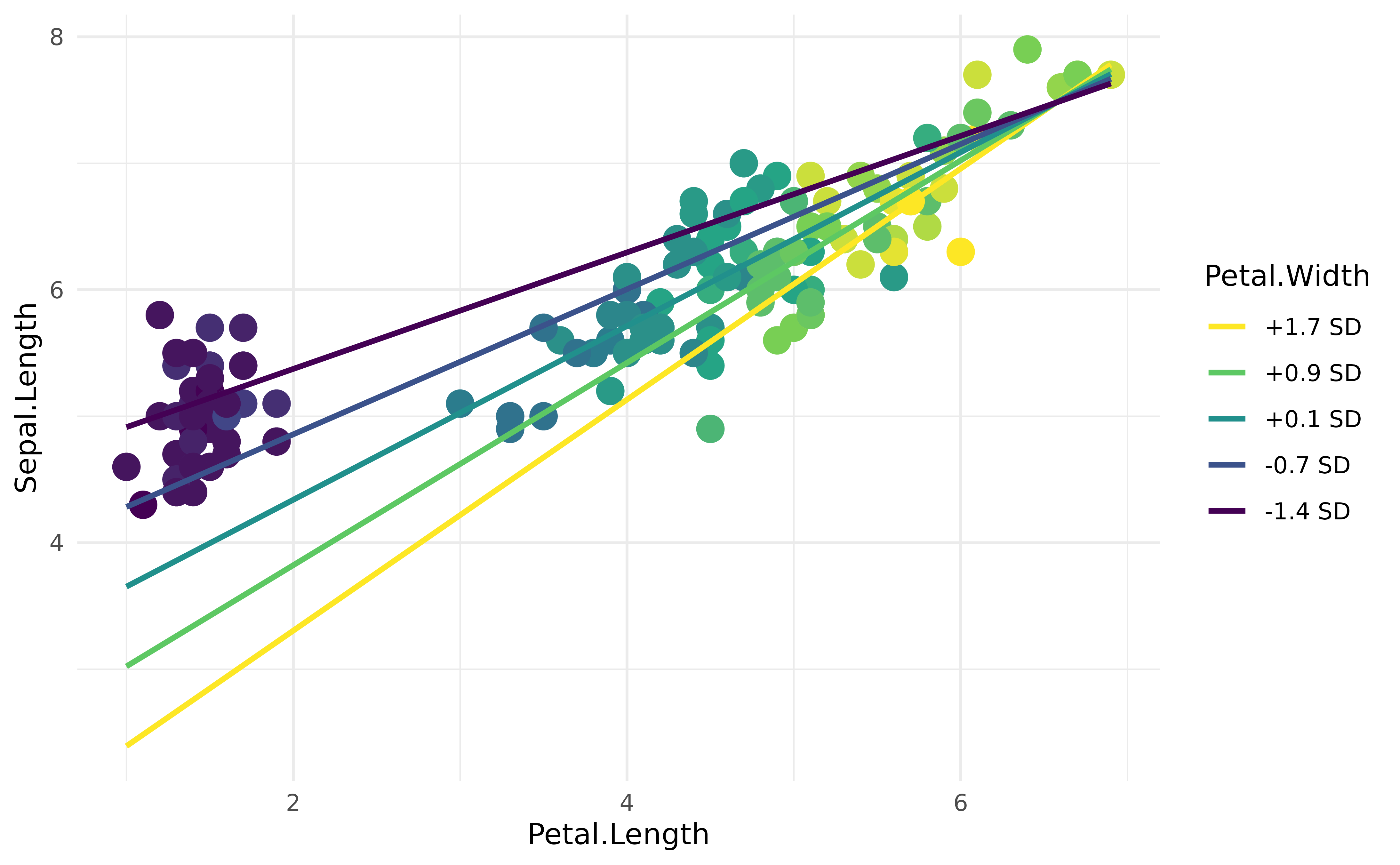
As the Petal.Width increases (becomes yellow), the
coefficient between Petal.Length and
Sepal.Length increases (the slope is more steep). Although,
as we can guess, this in fact captures the underlying effect of species…
but we’ll leave discussing the meaningfulness of your models to
you :)
get_datagrid() also runs directly on model objects
To illustrate this, let’s set up a general additive mixed
model (GAMM), where we are going to specify a smooth
term (a non-linear relationship; specified by s()
function) and some random effects structure.
library(gamm4)

model <- gamm4::gamm4(
  formula = Petal.Length ~ Petal.Width + s(Sepal.Length),
  random = ~ (1 | Species),
  data = iris
)
One can directly extract the visualization matrix for this model by entering the entire object into the function:
get_datagrid(model, length = 3, include_random = FALSE)> Visualisation Grid
>
> Petal.Width | Sepal.Length
> --------------------------
> 0.10 | 4.30
> 1.30 | 4.30
> 2.50 | 4.30
> 0.10 | 6.10
> 1.30 | 6.10
> 2.50 | 6.10
> 0.10 | 7.90
> 1.30 | 7.90
> 2.50 | 7.90We also skip the smooth term if we are interested only in the fixed effects:
get_datagrid(model, length = 3, include_random = FALSE, include_smooth = FALSE)> Visualisation Grid
>
> Petal.Width
> -----------
> 0.10
> 1.30
> 2.50
>
> Maintained constant: Sepal.LengthWe can also include random effects:
get_datagrid(model, length = 5, include_random = TRUE)> Visualisation Grid
>
> Petal.Width | Sepal.Length | Species
> ---------------------------------------
> 0.10 | 4.30 | setosa
> 0.10 | 5.20 | setosa
> 1.30 | 5.20 | versicolor
> 1.30 | 6.10 | versicolor
> 1.30 | 7.00 | versicolor
> 1.90 | 5.20 | virginica
> 2.50 | 5.20 | virginica
> 1.90 | 6.10 | virginica
> 2.50 | 6.10 | virginica
> 1.90 | 7.00 | virginica
> 2.50 | 7.00 | virginica
> 1.90 | 7.90 | virginica
> 2.50 | 7.90 | virginicaControlled standardized change
Although the plot above is nice, and all, we would like the standardized changes in SD to be smoother (e.g., by increments of 1 SD). This can be achieved by first requesting the values that we want, and then unstandardizing it.
Let’s use the same model as above, and then obtain a data grid with
specific values for Petal.Width.
vizdata <- lm(Sepal.Length ~ Petal.Length * Petal.Width, data = iris) |>
  get_datagrid(by = c("Petal.Length", "Petal.Width = seq(-3, 3)")) |>
  unstandardize(vizdata, select = "Petal.Width") |>
  estimate_relation(vizdata)

vizdata$Petal.Width <- effectsize::format_standardize(vizdata$Petal.Width, reference = iris$Petal.Width)

# 6. Plot
ggplot(iris, aes(x = Petal.Length, y = Sepal.Length)) +
  geom_point2(aes(fill = Petal.Width), shape = 21, size = 5) +
  geom_line(data = vizdata, aes(y = Predicted, color = Petal.Width), linewidth = 1) +
  scale_color_viridis_d(direction = -1) +
  scale_fill_viridis_c(guide = "none") +
  theme_minimal()