Case Study: Understanding your models
Source:vignettes/workflow_modelbased.Rmd
workflow_modelbased.RmdThis vignette demonstrates a typical workflow using easystats packages, with a logistic regression model as an example. We will explore how the modelbased package can help to better understand our model and how to interpret results.
Preparing the data and fitting a model
The very first step is usually importing and preparing some data
(recoding, re-shaping data and so on - the usual data wrangling tasks),
which is easily done using the datawizard package. In
this example, we use datawizard only for some minor recodings.
The coffee_data data set is included in the
modelbased package. The data set contains information
on the effect of coffee consumption on alertness over time. The outcome
variable is binary (alertness), and the predictor variables are coffee
consumption (treatment) and time.
library(datawizard) # for data management, e.g. recodings

data(coffee_data, package = "modelbased")

# dichotomize outcome variable
coffee_data$alertness <- categorize(coffee_data$alertness, lowest = 0)
# rename variable
coffee_data <- data_rename(coffee_data, select = c(treatment = "coffee"))

# model
model <- glm(alertness ~ treatment * time, data = coffee_data, family = binomial())
Exploring the model - model coefficients
Let’s start by examining the model coefficients. The package that
manages everything related to model coefficients is the
parameters package. We can use the
model_parameters() function to extract the coefficients
from the model. By setting exponentiate = TRUE, we can
obtain the odds ratios for the coefficients.
library(parameters)

# coefficients
model_parameters(model, exponentiate = TRUE)
#> Parameter                              | Odds Ratio |   SE |        95% CI |         z |      p
#> -----------------------------------------------------------------------------------------------
#> (Intercept)                            |       1.00 | 0.45 | [0.41,  2.44] | -1.54e-15 | > .999
#> treatment [control]                    |       0.33 | 0.23 | [0.08,  1.23] |     -1.61 | 0.108
#> time [noon]                            |       0.54 | 0.35 | [0.15,  1.90] |     -0.96 | 0.339
#> time [afternoon]                       |       3.00 | 2.05 | [0.81, 12.24] |      1.61 | 0.108
#> treatment [control] × time [noon]      |      10.35 | 9.85 | [1.66, 70.73] |      2.45 | 0.014
#> treatment [control] × time [afternoon] |       1.00 | 0.97 | [0.15,  6.74] | -6.10e-16 | > .999
#>
#> Uncertainty intervals (profile-likelihood) and p-values (two-tailed) computed using a Wald z-distribution approximation.
The model coefficients are difficult to interpret directly, in particular since we have an interaction effect. Instead, we should use the modelbased package to calculate adjusted predictions for the model.
Predicted probabilities - understanding the model
As we mentioned above, interpreting model results can be hard, and sometimes even misleading, if you only look at the regression coefficients. Instead, it is useful to estimate model-based means or probabilities for the outcome. Ab absolutely easy way to make interpretation easier is to use the modelbased package. You just need to provide your predictors of interest, so called focal terms.
Since we are interested in the interaction effect of coffee
consumption (treatment) on alertness depending on different times of the
day, we simply specify these two variables as focal terms in
the estimate_means() function. This function calculates
predictions on the response scale of the regression model. For logistic
regression models, predicted probabilities are calculated.
These refer to the adjusted probabilities of the outcome (higher
alertness) depending on the predictor variables (treatment and
time).
library(modelbased)

# predicted probabilities
predictions <- estimate_means(model, c("time", "treatment"))
predictions
#> Estimated Marginal Means
#>
#> time      | treatment | Probability |       95% CI
#> --------------------------------------------------
#> morning   | coffee    |        0.50 | [0.29, 0.71]
#> noon      | coffee    |        0.35 | [0.18, 0.57]
#> afternoon | coffee    |        0.75 | [0.52, 0.89]
#> morning   | control   |        0.25 | [0.11, 0.48]
#> noon      | control   |        0.65 | [0.43, 0.82]
#> afternoon | control   |        0.50 | [0.29, 0.71]
#>
#> Variable predicted: alertness
#> Predictors modulated: time, treatment
#> Predictions are on the response-scale.
We now see that high alertness was most likely for the
coffee group in the afternoon time (about 75%
probability of high alertness for the afternoon-coffee group).
We can also visualize these results, using the plot()
method. In short, this will give us a visual interpretation of the
model.
# plot predicted probabilities
plot(predictions)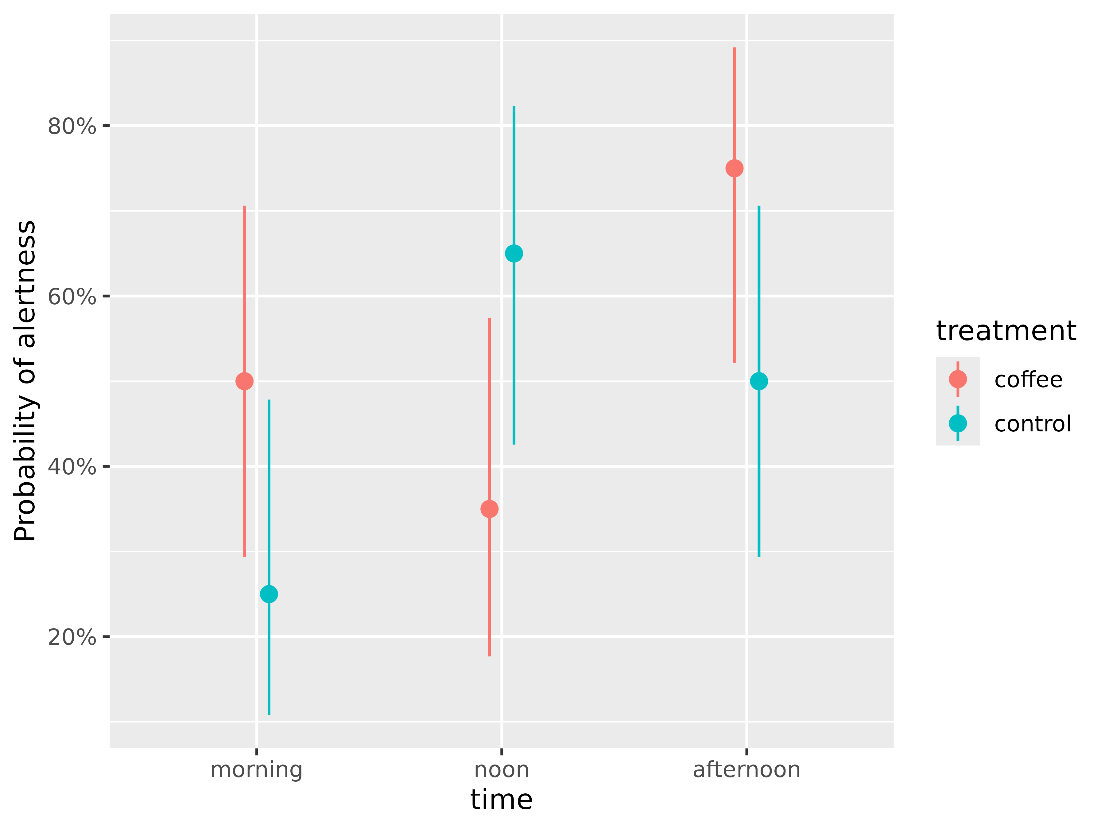
We can also see that the predicted probabilities of alertness are higher for participants who consumed coffee compared to those who did not, but only in the morning and in the afternoon. Furthermore, we see differences between the coffee and the control group at each time point - but are these differences statistically significant?
Pairwise comparisons - testing the differences
To check this, we finally use the estimate_contrasts()
function to perform pairwise comparisons of the predicted probabilities.
This function needs to know the variables that should be compared, or
contrasted. In a first step, we want to compare all levels of
the variables involved in our interaction term (our focal terms
from above).
# pairwise comparisons - quite long table
estimate_contrasts(model, c("time", "treatment"))
#> Marginal Contrasts Analysis
#>
#> Level1             | Level2            | Difference |   SE |        95% CI |        z |      p
#> ----------------------------------------------------------------------------------------------
#> morning, control   | morning, coffee   |      -0.25 | 0.15 | [-0.54, 0.04] |    -1.69 |  0.091
#> noon, coffee       | morning, coffee   |      -0.15 | 0.15 | [-0.45, 0.15] |    -0.97 |  0.332
#> noon, control      | morning, coffee   |       0.15 | 0.15 | [-0.15, 0.45] |     0.97 |  0.332
#> afternoon, coffee  | morning, coffee   |       0.25 | 0.15 | [-0.04, 0.54] |     1.69 |  0.091
#> afternoon, control | morning, coffee   |   1.11e-16 | 0.16 | [-0.31, 0.31] | 7.02e-16 | > .999
#> noon, coffee       | morning, control  |       0.10 | 0.14 | [-0.18, 0.38] |     0.69 |  0.488
#> noon, control      | morning, control  |       0.40 | 0.14 | [ 0.12, 0.68] |     2.78 |  0.005
#> afternoon, coffee  | morning, control  |       0.50 | 0.14 | [ 0.23, 0.77] |     3.65 | < .001
#> afternoon, control | morning, control  |       0.25 | 0.15 | [-0.04, 0.54] |     1.69 |  0.091
#> noon, control      | noon, coffee      |       0.30 | 0.15 | [ 0.00, 0.60] |     1.99 |  0.047
#> afternoon, coffee  | noon, coffee      |       0.40 | 0.14 | [ 0.12, 0.68] |     2.78 |  0.005
#> afternoon, control | noon, coffee      |       0.15 | 0.15 | [-0.15, 0.45] |     0.97 |  0.332
#> afternoon, coffee  | noon, control     |       0.10 | 0.14 | [-0.18, 0.38] |     0.69 |  0.488
#> afternoon, control | noon, control     |      -0.15 | 0.15 | [-0.45, 0.15] |    -0.97 |  0.332
#> afternoon, control | afternoon, coffee |      -0.25 | 0.15 | [-0.54, 0.04] |    -1.69 |  0.091
#>
#> Variable predicted: alertness
#> Predictors contrasted: time, treatment
#> p-values are uncorrected.
#> Contrasts are on the response-scale.
In the above output, we see all possible pairwise comparisons of the predicted probabilities. The table is quite long, but we can also group the comparisons, e.g. by the variable time.
# group comparisons by "time"
estimate_contrasts(model, "treatment", by = "time")
#> Marginal Contrasts Analysis
#>
#> Level1  | Level2 | time      | Difference |   SE |        95% CI |     z |     p
#> --------------------------------------------------------------------------------
#> control | coffee | morning   |      -0.25 | 0.15 | [-0.54, 0.04] | -1.69 | 0.091
#> control | coffee | noon      |       0.30 | 0.15 | [ 0.00, 0.60] |  1.99 | 0.047
#> control | coffee | afternoon |      -0.25 | 0.15 | [-0.54, 0.04] | -1.69 | 0.091
#>
#> Variable predicted: alertness
#> Predictors contrasted: treatment
#> p-values are uncorrected.
#> Contrasts are on the response-scale.
The output shows that the differences between the coffee and the control group are statistically significant only in the noon time.