Visualize effects and interactions

This vignette will present how to visualize the effects and interactions using estimate_relation().

Note that the statistically correct name of estimate_relation is estimate_expectation (which can be used as an alias), as it refers to expected predictions (read more).

Simple regression

Linear relationship

library(modelbased)

model <- glm(Sepal.Length ~ Sepal.Width, data = iris)

visualization_data <- estimate_relation(model)
head(visualization_data)

library(ggplot2)
library(see)
library(poorman)

visualization_data %>%
  ggplot(aes(x = Sepal.Width, y = Predicted)) +
  geom_ribbon(aes(ymin = CI_low, ymax = CI_high), alpha = 0.2) +
  geom_line() +
  see::theme_modern()

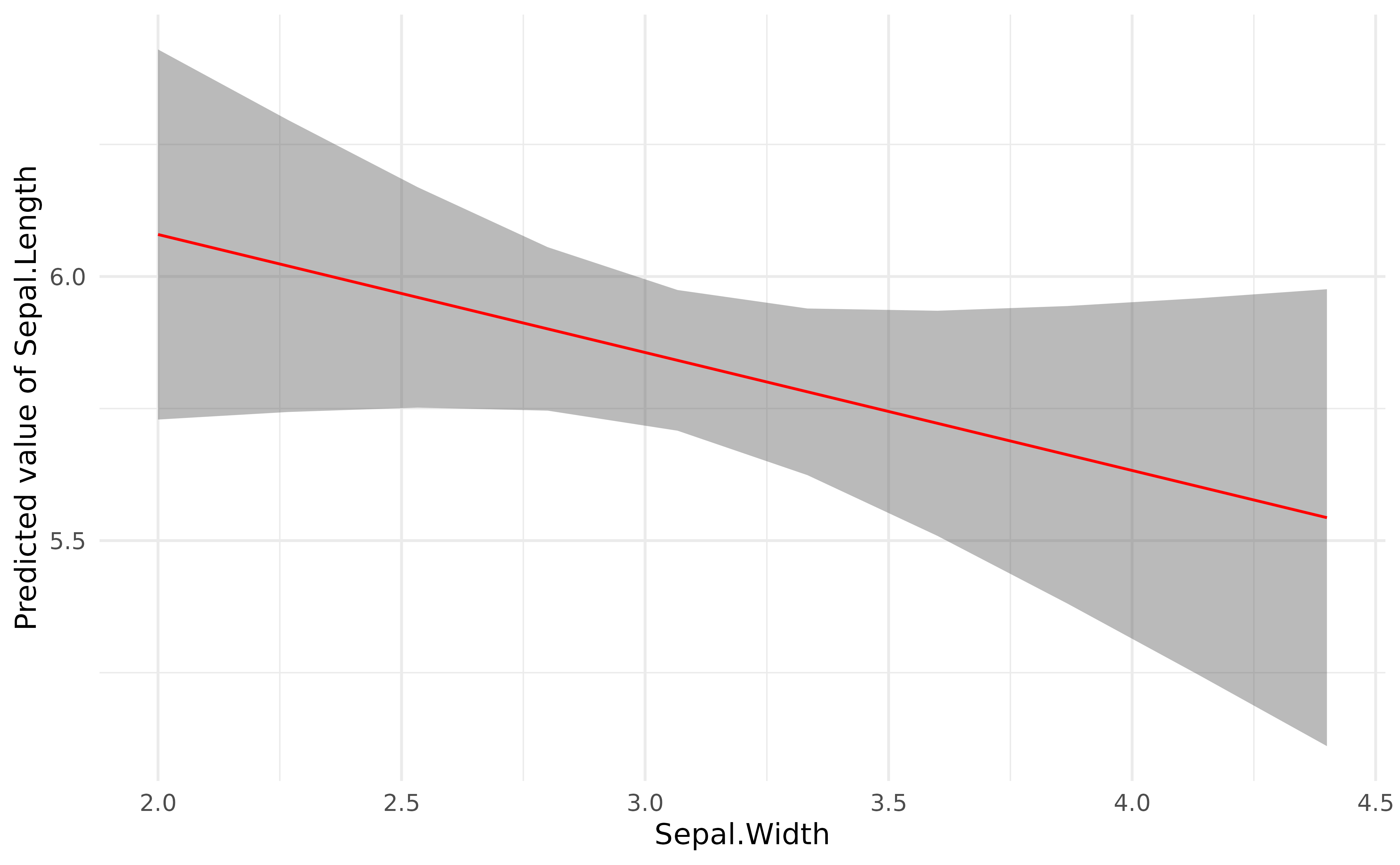
More complex regressions

Non-linear relationships

Note that non-linear relationships can be also described by linear approximations using describe_nonlinear.

Polynomial

glm(Sepal.Length ~ poly(Sepal.Width, 2), data = iris) %>%
  modelbased::estimate_relation(length = 50) %>%
  ggplot(aes(x = Sepal.Width, y = Predicted)) +
  geom_ribbon(aes(ymin = CI_low, ymax = CI_high), alpha = 0.2) +
  geom_line() +
  see::theme_modern()

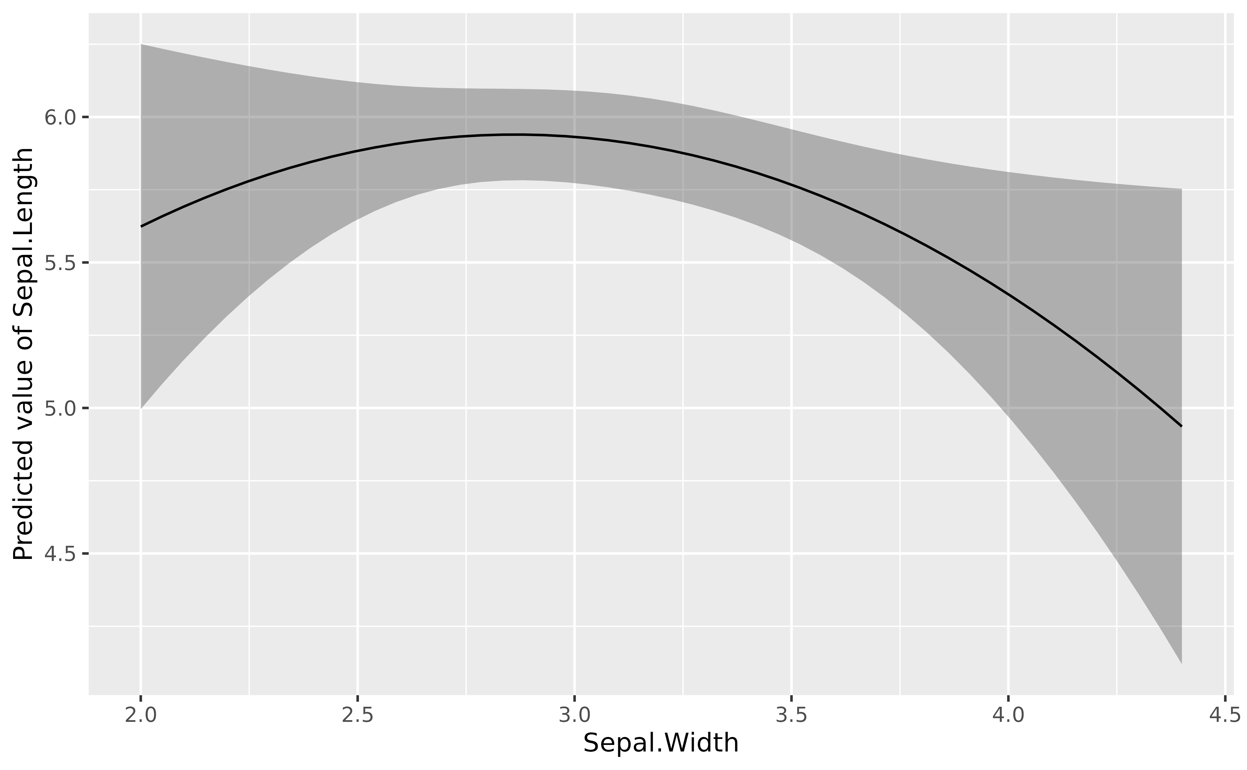
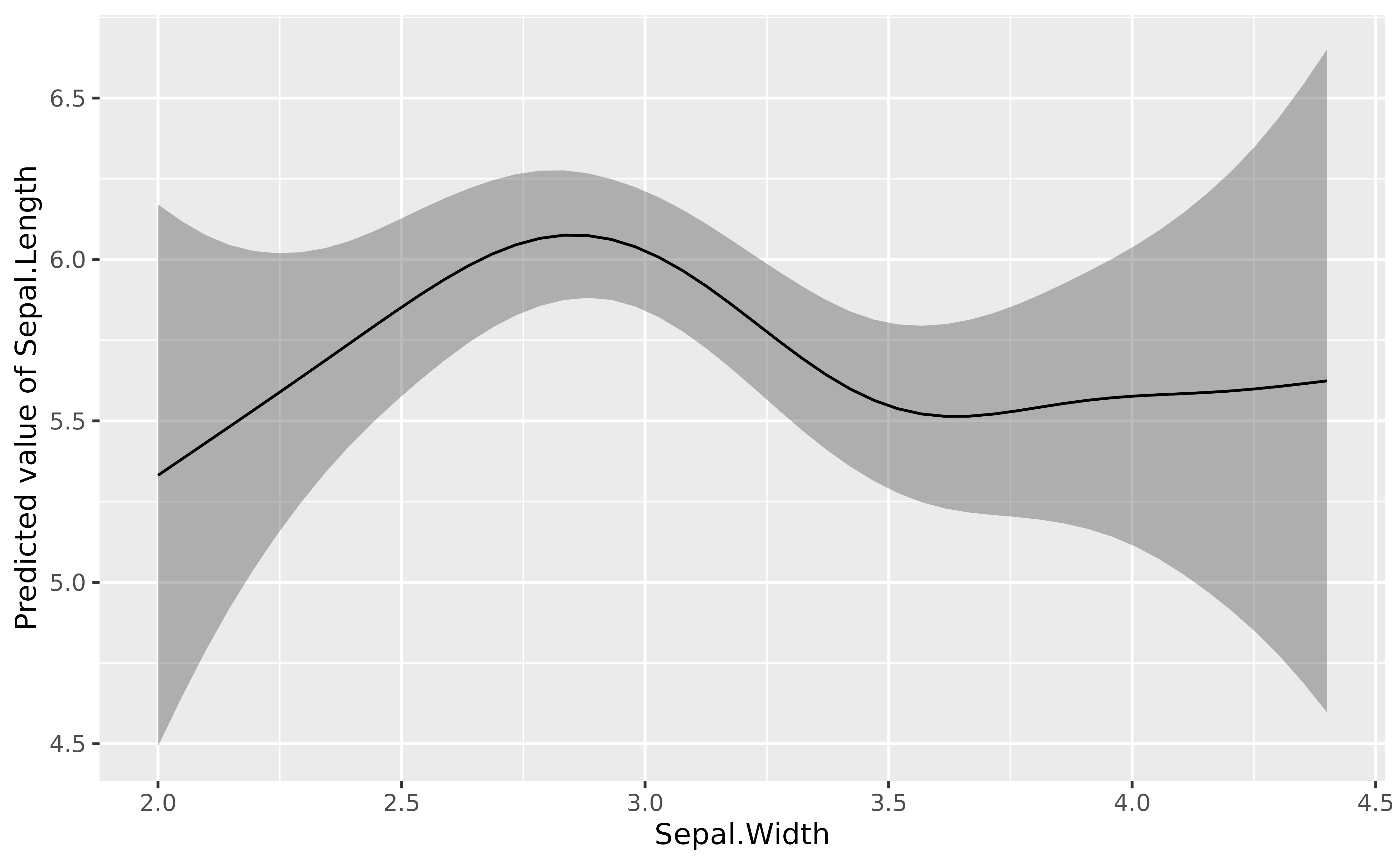
Additive Models

library(mgcv)

mgcv::gam(Sepal.Length ~ s(Sepal.Width), data = iris) %>%
  modelbased::estimate_relation(length = 50) %>%
  ggplot(aes(x = Sepal.Width, y = Predicted)) +
  geom_ribbon(aes(ymin = CI_low, ymax = CI_high), alpha = 0.2) +
  geom_line() +
  see::theme_modern()

Interactions

Interaction with a factor

TODO.

Interaction with another continuous variable

TODO.

Supported Models

TODO.

References