Context Effects: How the Environment Shapes the Individual
Source:vignettes/practical_context_effect.Rmd
practical_context_effect.RmdWhen analyzing longitudinal or clustered data, a standard mixed-effects model often blends two completely different processes into a single coefficient: the overall differences between individuals (or groups) and the acute fluctuations within an individual. However, separating these effects is just the first step. By evaluating them side-by-side, we can uncover a third, crucial piece of the puzzle: the context effect.
The context effect describes the additional influence that a broader
environment or a chronic baseline trait has on an individual,
independent of their immediate, momentary state (Rohrer and Murayama (2023)). By using the
demean() function to separate our time-varying predictors,
we can isolate the within- and between-components, evaluate them
independently, and formally test how the overarching context shapes
individual outcomes.
To understand the underlying problem of heterogeneity bias, demeaning (person-mean centering), and within/between effects in more detail, it is highly recommended to read this vignette first.
Note: Throughout this example, we use
display(format = "tt")to display table output in markdown format, using the tinytable package as the backend. See this vignette for more details on output displays.
Note: Because within-effects can vary across individuals, it is generally best practice to model them as random slopes. However, to keep this example simple, we have only included
timeas a random slope.
Sample data used in this vignette
library(parameters)
data("qol_cancer")- Variables:
-
QoL: Response (quality of life of patient) -
phq4: Patient Health Questionnaire, time-varying variable -
education: Educational level, time-invariant variable, co-variate -
ID: patient ID -
time: time-point of measurement
-
Computing the de-meaned and group-meaned variables
To calculate the within- and between-effects, we perform a special way of centering variables called demeaning. This “separates” the within-effect from a between-effect of a predictor.
library(datawizard)
qol_cancer <- demean(qol_cancer, select = c("phq4", "QoL"), by = "ID")
Now we have:
phq4_between: time-varying variable with the mean ofphq4across all time-points, for each patient (ID).phq4_within: the de-meaned time-varying variablephq4.
Calculating the within- and between effects using mixed models
First, we start with calculating the within- and between-effects from
phq4, before we move on to investigate the context
effects.
library(lme4)
mixed <- lmer(
  QoL ~ time + phq4_within + phq4_between + education + (1 + time | ID),
  data = qol_cancer
)
# effects = "fixed" will not display random effects, but split the
# fixed effects into its between- and within-effects components.
model_parameters(mixed, effects = "fixed") |> display(format = "tt")| Parameter | Coefficient | SE | 95% CI | t(554) | p |
|---|---|---|---|---|---|
| (Intercept) | 67.36 | 2.48 | (62.48, 72.23) | 27.15 | < .001 |
| time | 1.09 | 0.66 | (-0.21, 2.39) | 1.65 | 0.099 |
| phq4 within | -3.72 | 0.41 | (-4.52, -2.92) | -9.10 | < .001 |
| phq4 between | -6.13 | 0.52 | (-7.14, -5.11) | -11.84 | < .001 |
| education (mid) | 5.01 | 2.35 | (0.40, 9.62) | 2.14 | 0.033 |
| education (high) | 5.52 | 2.75 | (0.11, 10.93) | 2.00 | 0.046 |
Looking at the fixed effects output for the phq4
(Patient Health Questionnaire) variable, we can interpret the
coefficients as follows:
The Between-Effect (
phq4_between= -6.13): This captures the general, trait-like differences across patients. It answers the question: How does a patient’s overall average score affect their outcome compared to other patients? If Patient A has an overall averagephq4score that is 1 unit higher than Patient B’s average, we expect Patient A’s Quality of Life (QoL) to be 6.13 points lower on average than Patient B’s.The Within-Effect (
phq4_within= -3.72): This captures the state-like, time-to-time fluctuations for an individual. It answers the question: What happens when a patient deviates from their own baseline? If a patient scores 1 unit higher on thephq4at a specific time-point compared to their own personal average, their expected Quality of Life at that specific measurement decreases by an additional 3.72 points.
If we had entered phq4 into the model as a single,
uncentered variable, the resulting coefficient would be a weighted
average of these two distinct effects. This can be highly misleading, as
it obscures both the overarching patient-to-patient differences and the
specific time-to-time dynamics. Separating them provides a much clearer
picture of how psychological burden impacts quality of life on multiple
levels.
Context effect - contrasting within- and between-effects
Conceptually, when analyzing clustered or longitudinal data, we are looking at two distinct levels of influence:
Individual level (within-effect): What is the impact of an individual’s temporary deviation from their own group mean? This captures state-like fluctuations or acute changes.
Group level (between-effect): What is the impact of the group’s general environment or overall average, which affects all members equally? This captures trait-like, baseline differences or overarching environments.
The difference between these two effects is called the context effect. A context effect describes the additional influence that the general environment or baseline trait has on an individual, holding their raw, current state constant. It demonstrates that people with identical current, raw values (such as the exact same momentary income or symptom severity) face different outcomes depending on their baseline or the environment in which they live.
To test whether the within- and between-effects are significantly different from each other, we can estimate their contrast:
library(modelbased)
estimate_contrasts(mixed, c("phq4_within", "phq4_between")) |>
display(format = "tt")| Difference | SE | 95% CI | z | p |
|---|---|---|---|---|
| Variable predicted: QoL Predictors contrasted: phq4_within, phq4_between p-values are uncorrected. | ||||
| -2.41 | 0.66 | (-3.70, -1.12) | -3.66 | < .001 |
The output shows a significant contrast of -2.41 between the within- and between-effects. Since the between-effect in our model (-6.13) is stronger (more negative) than the within-effect (-3.72), the context-effect (Between minus Within) is -2.41.
What does this mean practically?
Imagine two patients who both report the exact same raw
phq4 score on a given day. However, Patient A generally
suffers from a higher overarching psychological burden (their personal
phq4 average is 1 unit higher than Patient B’s). The
context effect tells us that, despite experiencing the exact same
severity of symptoms today, Patient A’s expected Quality of Life is an
additional 2.41 points lower than Patient B’s simply because of their
higher baseline burden. The trait-like baseline carries an extra
“penalty” for the quality of life that goes beyond mere day-to-day
fluctuations.
Time trends of within- and between-effects
To investigate whether the impact of phq4 changes over
time, we can extend our model by adding interaction terms between the
time of measurement (time) and our two centered variables
(phq4_within and phq4_between).
mixed <- lmer(
  QoL ~ time * (phq4_within + phq4_between) + education + (1 + time | ID),
  data = qol_cancer
)
model_parameters(mixed, effects = "fixed") |> display(format = "tt")| Parameter | Coefficient | SE | 95% CI | t(552) | p |
|---|---|---|---|---|---|
| (Intercept) | 67.33 | 2.49 | (62.43, 72.23) | 26.99 | < .001 |
| time | 1.04 | 0.66 | (-0.25, 2.33) | 1.58 | 0.114 |
| phq4 within | -4.37 | 1.25 | (-6.81, -1.92) | -3.50 | < .001 |
| phq4 between | -4.70 | 0.96 | (-6.58, -2.82) | -4.90 | < .001 |
| education (mid) | 5.19 | 2.38 | (0.52, 9.87) | 2.18 | 0.029 |
| education (high) | 5.61 | 2.76 | (0.18, 11.04) | 2.03 | 0.043 |
| time × phq4 within | 0.33 | 0.61 | (-0.87, 1.52) | 0.54 | 0.592 |
| time × phq4 between | -0.66 | 0.37 | (-1.39, 0.07) | -1.77 | 0.077 |
The results table now shows us whether time has a moderating influence on our effects. To see this, we look at the two interaction terms at the bottom of the table:
Interaction
time × phq4_within: The coefficient (0.33) is small and not statistically significant (p = 0.592). This means that the negative effect of individual, temporary fluctuations remains largely stable over time. When a patient’s psychological burden acutely increases, their quality of life decreases to a very similar extent at any given time point.Interaction
time × phq4_between: This coefficient (-0.66) is also not statistically significant (p = 0.077). The negative sign suggests that the gap between patients potentially widens slightly over time. The “disadvantage” in quality of life experienced by patients with a generally high psychological baseline burden might further increase over the course of the study compared to less burdened patients.
These temporal dynamics can be best understood visually using Estimated Marginal Means. The generated plots confirm the statistical results from the table very clearly.
estimate_means(mixed, c("time", "phq4_within=[sd]")) |> plot()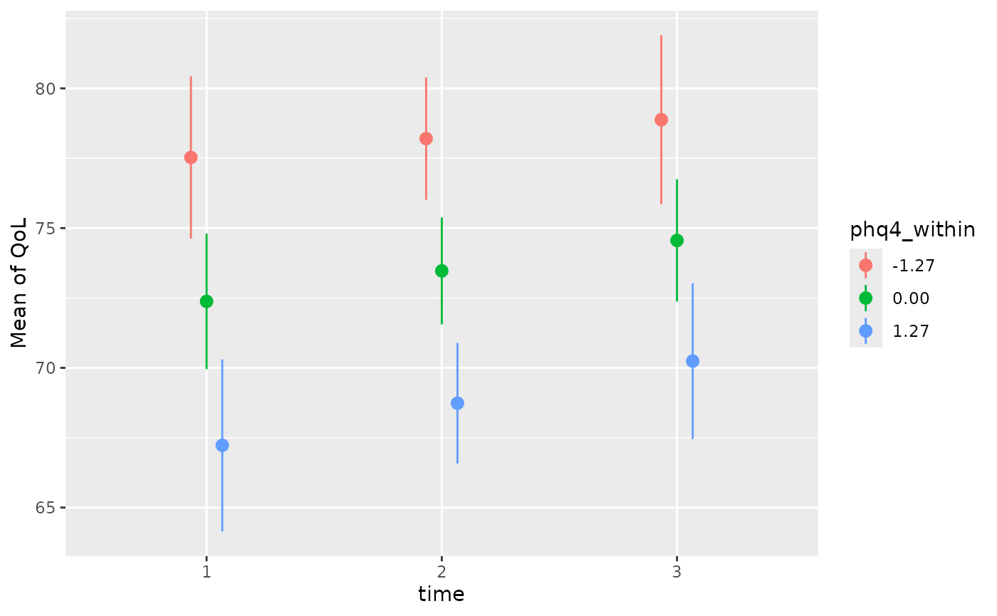
In the first plot (within-effects over time), the lines for
the different levels of phq4_within (mean as well as +/-
one standard deviation) run almost parallel. The constant distance
between the lines visualizes the lack of interaction: An acute increase
in psychological symptoms (shifting to the blue line) depresses the
quality of life uniformly across all time points.
estimate_means(mixed, c("time", "phq4_between=[sd]")) |> plot()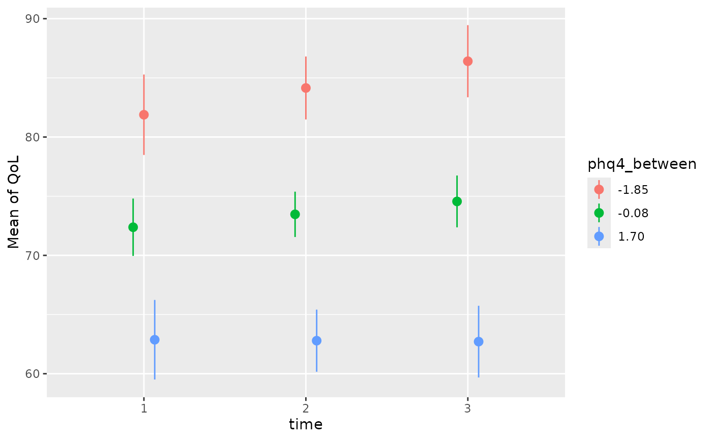
In the second plot (between-effects over time), a slight divergence of the lines is visible. While patients with a generally low burden (red line) experience a slight increase in their quality of life over time, the quality of life for patients with a generally high burden (blue line) stagnates at a lower level or even drops minimally.
Time trends of context effects
Finally, we might ask whether the context effect itself - the difference between the within- and between-effects - is stable, or if the “penalty” of a high baseline burden changes over the course of the study.
Before calculating the context effect directly, it is helpful to first look at the marginal effects (slopes) of both the within- and between-components separately at each time point. This helps us understand the underlying dynamics.
# average marginal effect of within-effect at each time point
estimate_slopes(mixed, "phq4_within", by = "time") |> display(format = "tt")| time | Slope | SE | 95% CI | t(552) | p |
|---|---|---|---|---|---|
| Marginal effects estimated for phq4_within Type of slope was dY/dX | |||||
| 1 | -4.04 | 0.70 | (-5.42, -2.66) | -5.77 | < .001 |
| 2 | -3.71 | 0.41 | (-4.52, -2.91) | -9.07 | < .001 |
| 3 | -3.39 | 0.76 | (-4.89, -1.88) | -4.43 | < .001 |
# average marginal effect of between-effect at each time point
estimate_slopes(mixed, "phq4_between", by = "time") |> display(format = "tt")| time | Slope | SE | 95% CI | t(552) | p |
|---|---|---|---|---|---|
| Marginal effects estimated for phq4_between Type of slope was dY/dX | |||||
| 1 | -5.36 | 0.68 | (-6.69, -4.03) | -7.92 | < .001 |
| 2 | -6.02 | 0.52 | (-7.04, -4.99) | -11.52 | < .001 |
| 3 | -6.68 | 0.60 | (-7.87, -5.49) | -11.05 | < .001 |
Looking at these separate slopes reveals two opposing trends. The
acute impact of a temporary symptom spike (phq4_within)
slightly decreases in magnitude over time (shifting from -4.04 at Time 1
to -3.39 at Time 3). Conversely, the detrimental impact of a chronically
high baseline burden (phq4_between) becomes progressively
more severe, worsening from -5.36 to -6.68.
Because these two effects drift further apart over time, we can now formally test their difference — the context effect — by calculating the marginal contrasts at each specific time point.
estimate_contrasts(
  mixed,
  c("phq4_within", "phq4_between"),
  by = "time"
) |>
display(format = "tt")| time | Difference | SE | 95% CI | z | p |
|---|---|---|---|---|---|
| Variable predicted: QoL Predictors contrasted: phq4_within, phq4_between p-values are uncorrected. | |||||
| 1 | -1.32 | 1.00 | (-3.28, 0.65) | -1.32 | 0.188 |
| 2 | -2.31 | 0.66 | (-3.60, -1.01) | -3.48 | < .001 |
| 3 | -3.29 | 0.99 | (-5.22, -1.36) | -3.34 | < .001 |
The contrast analysis reveals a clear and interesting trajectory: the context effect grows substantially stronger as time progresses.
At Time 1 (Baseline): The difference between the within- and between-effect is relatively small (-1.32) and not statistically significant (p = 0.188). This indicates that at the beginning of the observations, it does not matter much whether a patient’s psychological burden is acute (a temporary spike) or chronic (a generally high baseline). The immediate impact on their Quality of Life is very similar.
At Time 2 and Time 3: As the study progresses, the contrast becomes highly significant and the gap widens (an absolute increase to 2.31, then 3.29).
What does this mean practically?
Over time, having a chronically high baseline of psychological symptoms (the trait-level burden) becomes increasingly detrimental compared to merely experiencing a temporary, acute spike in symptoms. While patients might be able to buffer or cope with an acute worsening of their mental state similarly well at any point, the cumulative “wear and tear” of a chronically high burden takes an increasing toll on their quality of life as time goes on.
Testing the Change in the Context Effect Over Time
While the previous table showed the context effect at each specific time point, we also need to formally test whether the change in this effect over time is statistically significant. We can do this by computing pairwise comparisons of the context effect across the different time points.
estimate_contrasts(
  mixed,
  c("phq4_within", "phq4_between", "time")
) |>
display(format = "tt")| Level1 | Level2 | Difference | SE | 95% CI | z | p |
|---|---|---|---|---|---|---|
| Variable predicted: QoL Predictors contrasted: phq4_within, phq4_between p-values are uncorrected. | ||||||
| 2 | 1 | -0.99 | 0.74 | (-2.44, 0.47) | -1.33 | 0.183 |
| 3 | 1 | -1.97 | 1.48 | (-4.88, 0.93) | -1.33 | 0.183 |
| 3 | 2 | -0.99 | 0.74 | (-2.44, 0.47) | -1.33 | 0.183 |
This pairwise comparison table adds a crucial statistical caveat to our visual and descriptive observations. The Difference column here represents the mathematical change in the size of the context effect between two specific time points (e.g., the context effect decreased by 0.99 points from Time 1 to Time 2).
However, looking at the statistics, you will notice that the estimated difference between any two adjacent time points is exactly identical, yielding the exact same standard error and p-value.
This uniformity is a direct mathematical consequence of our model assuming a strictly linear time trend. Under a linear assumption, the rate of change (the slope) is constrained to be constant. Therefore, the estimated change in the context effect from Time 1 to Time 2 is forced to be exactly the same as the change from Time 2 to Time 3. These point-to-point comparisons would only vary if we had modeled time non-linearly (for instance, by adding a quadratic term).
Because a linear model yields constant step-by-step changes, testing these identical individual intervals is often less informative. To test whether the context effect meaningfully changes over time overall, it is more appropriate to evaluate the average contrast of the slopes across the entire study period. To do this, we calculate the contrast between the within- and between-effects without stratifying by time.
estimate_contrasts(mixed, c("phq4_within", "phq4_between")) |>
display(format = "tt")| Difference | SE | 95% CI | z | p |
|---|---|---|---|---|
| Variable predicted: QoL Predictors contrasted: phq4_within, phq4_between p-values are uncorrected. | ||||
| -2.31 | 0.66 | (-3.60, -1.01) | -3.48 | < .001 |
What does this mean practically?
The highly significant overall contrast (-2.31, p < .001) confirms that a substantial context effect is at play throughout the entire observation period.
In clinical terms, while an acute, temporary spike in psychological symptoms (the within-effect) definitely harms a patient’s quality of life, carrying a chronically high baseline burden (the between-effect) takes a significantly heavier toll. A patient who generally suffers from high psychological distress faces an overarching “trait penalty” that consistently depresses their quality of life more severely than mere day-to-day fluctuations would suggest.
Trends of Context Effects Across Educational Levels
To explore whether socioeconomic factors influence these dynamics, we can test if the context effect varies across different educational backgrounds. A reasonable assumption might be that highly educated individuals possess more resources (cognitive, financial, or social) and thus cope better with psychological burden.
To formally test this, we extend our model to include a three-way
interaction between time, education, and our
centered phq4 variables.
mixed <- lmer(
  QoL ~ time * education * (phq4_within + phq4_between) + (1 + time | ID),
  data = qol_cancer
)
estimate_contrasts(
  mixed,
  c("phq4_within", "phq4_between"),
  by = "education"
) |>
display(format = "tt")| education | Difference | SE | 95% CI | z | p |
|---|---|---|---|---|---|
| Variable predicted: QoL Predictors contrasted: phq4_within, phq4_between p-values are uncorrected. | |||||
| low | -1.69 | 1.30 | (-4.24, 0.85) | -1.30 | 0.192 |
| mid | -3.92 | 0.87 | (-5.64, -2.21) | -4.49 | < .001 |
| high | 1.76 | 1.84 | (-1.84, 5.36) | 0.96 | 0.337 |
The marginal contrasts analysis yields nuanced results that add an important layer to our understanding of the context effect:
- Low Education: The contrast (-1.69) is not statistically significant (p = 0.192). For these patients, there is no meaningful difference between an acute symptom spike and a chronically high baseline. Both states depress their quality of life similarly.
- Mid Education: The contrast (-3.92) is large and highly significant (p < .001). This group actually drives the overall context effect we observed in the previous models. For middle-educated patients, a chronically high psychological burden carries a massive additional penalty compared to a temporary acute spike (their quality of life is decreasing by 3.92 points).
- High Education: Interestingly, the contrast reverses its sign (1.76) but is not statistically significant (p = 0.337). This indicates that for highly educated patients, the context effect disappears entirely.
What does this mean practically?
The hypothesis that highly educated people “fare better” is supported here, but in a very specific, mechanistic way. While we would need to look at the main effects to see if their absolute Quality of Life is higher, this contrast analysis tells us how they process psychological burden.
Highly educated patients appear to be buffered against the specific “chronic penalty”. For them, carrying a chronic baseline burden is no more destructive to their quality of life than experiencing an acute, temporary spike. They likely possess the resources needed to manage a chronic psychological load without letting it compound into an overarching environmental penalty.
Conversely, the middle-educated group represents a highly vulnerable population regarding these dynamics. They suffer disproportionately from a chronically high baseline burden.
Are the Trends of Context Effects Significantly Different Between Groups?
In the previous step, we observed that the context effect seemed to be entirely driven by the middle-educated group, while highly educated patients appeared to be buffered against it. However, to rigorously test whether the size of the context effect is statistically different between these groups, we need to compute pairwise comparisons across the educational levels.
We can do this by adding the grouping variable
(education) as a third term to our contrast statement.
estimate_contrasts(
  mixed,
  c("phq4_within", "phq4_between", "education")
) |>
display(format = "tt")| Level1 | Level2 | Difference | SE | 95% CI | z | p |
|---|---|---|---|---|---|---|
| Variable predicted: QoL Predictors contrasted: phq4_within, phq4_between p-values are uncorrected. | ||||||
| mid | low | -2.23 | 1.57 | (-5.30, 0.84) | -1.42 | 0.154 |
| high | low | 3.46 | 2.25 | (-0.95, 7.86) | 1.54 | 0.124 |
| high | mid | 5.69 | 2.03 | ( 1.70, 9.67) | 2.80 | 0.005 |
The output now displays the mathematical difference in the size of the context effect between two specific groups.
- Mid vs. Low (p = 0.154) & High vs. Low (p = 0.124): The differences involving the low-education group are not statistically significant. The confidence intervals are quite wide, suggesting high variance or a smaller sample size within this specific intersection of the data.
- High vs. Mid (Difference = 5.69, p = 0.005): This is the crucial finding. The context effect for the highly educated group is significantly larger (by 5.69 points) than for the middle-educated group.
What does this mean practically?
This pairwise comparison formally solidifies our previous suspicion: The buffering effect of higher education is statistically robust.
It proves that the “chronic penalty” for long-term psychological burden does not hit everyone equally. The structural or psychological advantages possessed by the highly educated group (such as better access to support networks, financial stability, or coping resources) create a mathematically significant difference in how chronic distress is processed. Compared directly to the middle-educated tier—who bear the full weight of the context effect—highly educated patients are significantly better protected from the cumulative “wear and tear” of a chronically high baseline burden.