Group-specific parameters of mixed models random effects — estimate

Extract random parameters of each individual group in the context of mixed models, commonly referred to as BLUPs (Best Linear Unbiased Predictors). Can be reshaped to be of the same dimensions as the original data, which can be useful to add the random effects to the original data.

Usage

estimate_grouplevel(model, ...)

# Default S3 method
estimate_grouplevel(model, type = "random", ...)

# S3 method for class 'brmsfit'
estimate_grouplevel(
  model,
  type = "random",
  dispersion = TRUE,
  test = NULL,
  diagnostic = NULL,
  ...
)

reshape_grouplevel(x, ...)

# S3 method for class 'estimate_grouplevel'
reshape_grouplevel(x, indices = "all", group = NULL, ...)

Arguments

model

A mixed model with random effects.

...

Other arguments passed to parameters::model_parameters() or estimate_means().

type

String, describing the type of estimates that should be returned. Can be "random", "total", or "marginal" (experimental).

If "random" (default), the coefficients correspond to the conditional estimates of the random effects (as they are returned by lme4::ranef()). They typically correspond to the deviation of each individual group from their fixed effect (assuming the random effect is also included as a fixed effect). As such, a coefficient close to 0 means that the participants' effect is the same as the population-level effect (in other words, it is "in the norm"). These estimates are typically the same as the "total" ones, but are simply expressed on a different scale: relative to the fixed effect vs. absolute coefficient values.
If "total", it will return the sum of the random effect and its corresponding fixed effects, which internally relies on the coef() method (see ?coef.merMod). Note that type = "total" yet does not return uncertainty indices (such as SE and CI) for models from lme4 or glmmTMB, as the necessary information to compute them is not yet available. However, for Bayesian models, it is possible to compute them.
If "marginal" (experimental), it returns marginal group-level estimates. The random intercepts are computed using marginal means (see estimate_means()), and the random slopes using marginal effects (see estimate_slopes()). This method does not directly extract the parameters estimated by the model, but recomputes them using model predictions. By default, the function uses "typical" marginalization (estimate = "typical"). This results in estimates closely comparable to that when type = "total" (and identical to it when continuous predictors are mean-centered). Setting estimate = "average" instead returns each group's actual average predicted outcome, based on that group's own observed predictor distribution rather than a shared reference point (see below for details on this distinction). One benefit of "marginal" over "total"/"random" is interpretability for non-linear models (e.g. logistic or count GLMMs), since predictions are expressed on the response scale rather than the link scale. Note that group-level estimates here are not technically "intercepts" or model parameters, but marginal average levels and effects.

dispersion, test, diagnostic

Arguments passed to parameters::model_parameters() for Bayesian models. By default, it won't return significance or diagnostic indices (as it is not typically very useful).

x

The output of estimate_grouplevel().

indices

A character vector containing the indices (i.e., which columns) to extract (e.g., "Coefficient", "Median").

group

The name of the random factor to select as string value (e.g., "Participant", if the model was y ~ x + (1|Participant).

Details

Benefits of model-based group-level estimates:

Unlike raw group means, BLUPs apply shrinkage: they are a compromise between the group estimate and the population estimate. This improves generalizability and prevents overfitting.

What group-level estimates tell you:

Imagine the two following scenarios:

Scenario 1: A reaction time task where each trial is assigned to a difficulty condition. It is a manipulated, balanced experimental condition. We have model like rt ~ Condition + (Condition | Participant), where Condition (1-5) is assigned by the experiment, so every participant completes the same set of levels in the same proportions.
Scenario 2: A reaction time task where participants rate each trial according to their own self-reported confidence - e.g. rt ~ Confidence + (Confidence | Participant), where Confidence (1-5) is generated by the participant, and so varies by participant both in its average level (some participants report high confidence overall, some low) and in how strongly it relates to RT (some have strong metacognition - a steep slope - others don't).

In Scenario 1, interpretation is straightforward and largely insensitive to which method is used ("random", "total", or "marginal", with either estimate option). Because every participant is exposed to the same balanced set of Condition levels, each participant's own mean Condition already equals the grand mean. There is no meaningful difference between evaluating at a shared reference point versus at each participant's own observed values, so all approaches converge on essentially the same answer: the random intercept values tell us how fast or slow each participant is overall, and the random slopes of Condition tell us how strongly each participant's RT is affected by increasing difficulty, relative to the population-level effect of Condition.

In Scenario 2, this is no longer true, and the choice of method changes what the random intercepts and slopes mean. Two families of estimates emerge:

type = "total"/"random", and type = "marginal" with estimate = "typical" (default), all evaluate every participant at one shared reference point (the model's intercept, or the grand mean of Confidence, respectively). These target each participant's intrinsic characteristics - their personal regression line itself - independently of how often they happened to report a given confidence level. The trade-off is that this can be a counterfactual quantity: for a participant whose confidence ratings rarely approach the grand mean, "their predicted RT at average confidence" extrapolates beyond what they actually reported. The random intercept tells us how fast or slow this participant would intrinsically be at the same (hypothetical) confidence level, and the random slope of Confidence tells us how strongly their RT is intrinsically tied to their own confidence ratings - both independent of how often they happen to report high or low confidence.
type = "marginal" with estimate = "average" instead evaluates each participant using their own observed distribution of Confidence. This avoids extrapolation, but it now conflates the participant's intrinsic regression parameters with their personal response style: a chronically high-confidence participant with a steep slope will get a marginal intercept reflecting both their baseline speed and their tendency to report high confidence, entangled into a single number. It is no longer a controlled, like-for-like comparison across participants. The random intercept tells us how fast or slow this participant actually was, on average, across the confidence levels they actually reported while the random slope tells us how strongly their RT tracks their own confidence ratings.

As a rule of thumb: use "total", "random", or "marginal" with estimate = "typical" when you want each group's intrinsic characteristics, comparable on equal footing across groups. Use "marginal" with estimate = "average" when you want each group's actual, as-observed outcome, accepting that it may reflect a mix of intrinsic effect and exposure or response style, especially when the predictors values vary across random factor levels.

Examples

# lme4 model
data(mtcars)
model <- lme4::lmer(mpg ~ hp + (1 | carb), data = mtcars)
random <- estimate_grouplevel(model)

# Show group-specific effects
random
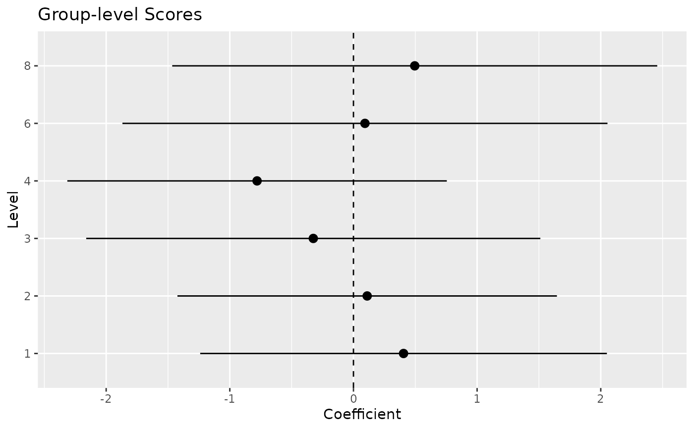
#> Group | Level | Parameter   | Coefficient |   SE |        95% CI
#> ----------------------------------------------------------------
#> carb  | 1     | (Intercept) |        0.41 | 0.84 | [-1.24, 2.05]
#> carb  | 2     | (Intercept) |        0.11 | 0.78 | [-1.42, 1.65]
#> carb  | 3     | (Intercept) |       -0.32 | 0.94 | [-2.16, 1.51]
#> carb  | 4     | (Intercept) |       -0.78 | 0.78 | [-2.31, 0.75]
#> carb  | 6     | (Intercept) |        0.09 | 1.00 | [-1.87, 2.05]
#> carb  | 8     | (Intercept) |        0.50 | 1.00 | [-1.47, 2.46]

# Visualize random effects
plot(random)


# Reshape to wide data...
reshaped <- reshape_grouplevel(random, group = "carb", indices = c("Coefficient", "SE"))

# ...and can be easily combined with the original data
alldata <- merge(mtcars, reshaped)

# overall coefficients
r_tot <- estimate_grouplevel(model, type = "total")
cor(r_tot$Coefficient, random$Coefficient) # r = 1 (just a scale difference)
#> [1] 1

# marginal coefficients
r_mar <- estimate_grouplevel(model, type = "marginal")
cor(r_mar$Coefficient, r_tot$Coefficient)
#> [1] 1