Probability of Direction (pd)

Compute the Probability of Direction (pd, also known as the Maximum Probability of Effect - MPE). This can be interpreted as the probability that a parameter (described by its full confidence, or "compatibility" interval) is strictly positive or negative (whichever is the most probable). Although differently expressed, this index is fairly similar (i.e., is strongly correlated) to the frequentist p-value (see 'Details').

Usage

# S3 method for class 'lm'
p_direction(x, ci = 0.95, method = "direct", null = 0, ...)

Arguments

x: A statistical model.
ci: Confidence Interval (CI) level. Default to 0.95 (95%).
method: Can be "direct" or one of methods of estimate_density(), such as "kernel", "logspline" or "KernSmooth". See details.
null: The value considered as a "null" effect. Traditionally 0, but could also be 1 in the case of ratios of change (OR, IRR, ...).
...: Arguments passed to other methods, e.g. ci(). Arguments like vcov or vcov_args can be used to compute confidence intervals using a specific variance-covariance matrix for the standard errors.

Value

A data frame.

What is the pd?

The Probability of Direction (pd) is an index of effect existence, representing the certainty with which an effect goes in a particular direction (i.e., is positive or negative / has a sign), typically ranging from 0.5 to 1 (but see next section for cases where it can range between 0 and 1). Beyond its simplicity of interpretation, understanding and computation, this index also presents other interesting properties:

Like other posterior-based indices, pd is solely based on the posterior distributions and does not require any additional information from the data or the model (e.g., such as priors, as in the case of Bayes factors).
It is robust to the scale of both the response variable and the predictors.
It is strongly correlated with the frequentist p-value, and can thus be used to draw parallels and give some reference to readers non-familiar with Bayesian statistics (Makowski et al., 2019).

Relationship with the p-value

In most cases, it seems that the pd has a direct correspondence with the frequentist one-sided p-value through the formula (for two-sided p): p = 2 * (1 - p_d) Thus, a two-sided p-value of respectively .1, .05, .01 and .001 would correspond approximately to a pd of 95%, 97.5%, 99.5% and 99.95%. See pd_to_p() for details.

Possible Range of Values

The largest value pd can take is 1 - the posterior is strictly directional. However, the smallest value pd can take depends on the parameter space represented by the posterior.

For a continuous parameter space, exact values of 0 (or any point null value) are not possible, and so 100% of the posterior has some sign, some positive, some negative. Therefore, the smallest the pd can be is 0.5 - with an equal posterior mass of positive and negative values. Values close to 0.5 cannot be used to support the null hypothesis (that the parameter does not have a direction) is a similar why to how large p-values cannot be used to support the null hypothesis (see pd_to_p(); Makowski et al., 2019).

For a discrete parameter space or a parameter space that is a mixture between discrete and continuous spaces, exact values of 0 (or any point null value) are possible! Therefore, the smallest the pd can be is 0 - with 100% of the posterior mass on 0. Thus values close to 0 can be used to support the null hypothesis (see van den Bergh et al., 2021).

Examples of posteriors representing discrete parameter space:

When a parameter can only take discrete values.
When a mixture prior/posterior is used (such as the spike-and-slab prior; see van den Bergh et al., 2021).
When conducting Bayesian model averaging (e.g., weighted_posteriors() or brms::posterior_average).

Statistical inference - how to quantify evidence

There is no standardized approach to drawing conclusions based on the available data and statistical models. A frequently chosen but also much criticized approach is to evaluate results based on their statistical significance (Amrhein et al. 2017).

A more sophisticated way would be to test whether estimated effects exceed the "smallest effect size of interest", to avoid even the smallest effects being considered relevant simply because they are statistically significant, but clinically or practically irrelevant (Lakens et al. 2018, Lakens 2024).

A rather unconventional approach, which is nevertheless advocated by various authors, is to interpret results from classical regression models in terms of probabilities, similar to the usual approach in Bayesian statistics (Greenland et al. 2022; Rafi and Greenland 2020; Schweder 2018; Schweder and Hjort 2003; Vos 2022).

The parameters package provides several options or functions to aid statistical inference. These are, for example:

equivalence_test(), to compute the (conditional) equivalence test for frequentist models
p_significance(), to compute the probability of practical significance, which can be conceptualized as a unidirectional equivalence test
p_function(), or consonance function, to compute p-values and compatibility (confidence) intervals for statistical models
the pd argument (setting pd = TRUE) in model_parameters() includes a column with the probability of direction, i.e. the probability that a parameter is strictly positive or negative. See bayestestR::p_direction() for details. If plotting is desired, the p_direction() function can be used, together with plot().
the s_value argument (setting s_value = TRUE) in model_parameters() replaces the p-values with their related S-values (Rafi and Greenland 2020)
finally, it is possible to generate distributions of model coefficients by generating bootstrap-samples (setting bootstrap = TRUE) or simulating draws from model coefficients using simulate_model(). These samples can then be treated as "posterior samples" and used in many functions from the bayestestR package.

Most of the above shown options or functions derive from methods originally implemented for Bayesian models (Makowski et al. 2019). However, assuming that model assumptions are met (which means, the model fits well to the data, the correct model is chosen that reflects the data generating process (distributional model family) etc.), it seems appropriate to interpret results from classical frequentist models in a "Bayesian way" (more details: documentation in p_function()).

References

Amrhein, V., Korner-Nievergelt, F., and Roth, T. (2017). The earth is flat (p > 0.05): Significance thresholds and the crisis of unreplicable research. PeerJ, 5, e3544. doi:10.7717/peerj.3544
Greenland S, Rafi Z, Matthews R, Higgs M. To Aid Scientific Inference, Emphasize Unconditional Compatibility Descriptions of Statistics. (2022) https://arxiv.org/abs/1909.08583v7 (Accessed November 10, 2022)
Lakens, D. (2024). Improving Your Statistical Inferences (Version v1.5.1). Retrieved from https://lakens.github.io/statistical_inferences/. doi:10.5281/ZENODO.6409077
Lakens, D., Scheel, A. M., and Isager, P. M. (2018). Equivalence Testing for Psychological Research: A Tutorial. Advances in Methods and Practices in Psychological Science, 1(2), 259–269. doi:10.1177/2515245918770963
Makowski, D., Ben-Shachar, M. S., Chen, S. H. A., and Lüdecke, D. (2019). Indices of Effect Existence and Significance in the Bayesian Framework. Frontiers in Psychology, 10, 2767. doi:10.3389/fpsyg.2019.02767
Rafi Z, Greenland S. Semantic and cognitive tools to aid statistical science: replace confidence and significance by compatibility and surprise. BMC Medical Research Methodology (2020) 20:244.
Schweder T. Confidence is epistemic probability for empirical science. Journal of Statistical Planning and Inference (2018) 195:116–125. doi:10.1016/j.jspi.2017.09.016
Schweder T, Hjort NL. Frequentist analogues of priors and posteriors. In Stigum, B. (ed.), Econometrics and the Philosophy of Economics: Theory Data Confrontation in Economics, pp. 285-217. Princeton University Press, Princeton, NJ, 2003
Vos P, Holbert D. Frequentist statistical inference without repeated sampling. Synthese 200, 89 (2022). doi:10.1007/s11229-022-03560-x

Examples

data(qol_cancer)
model <- lm(QoL ~ time + age + education, data = qol_cancer)
p_direction(model)
#> Probability of Direction (null: 0)
#> 
#> Parameter     |         95% CI |     pd
#> ---------------------------------------
#> (Intercept)   | [58.46, 69.28] |   100%
#> time          | [-1.07,  2.85] | 81.46%
#> age           | [-0.32,  0.37] | 55.95%
#> educationmid  | [ 4.43, 13.09] | 99.99%
#> educationhigh | [ 9.33, 19.38] |   100%

# based on heteroscedasticity-robust standard errors
p_direction(model, vcov = "HC3")
#> Probability of Direction (null: 0)
#> 
#> Parameter     |         95% CI |     pd
#> ---------------------------------------
#> (Intercept)   | [58.33, 69.41] |   100%
#> time          | [-1.13,  2.90] | 80.70%
#> age           | [-0.33,  0.38] | 55.36%
#> educationmid  | [ 4.21, 13.31] |   100%
#> educationhigh | [ 9.37, 19.34] |   100%

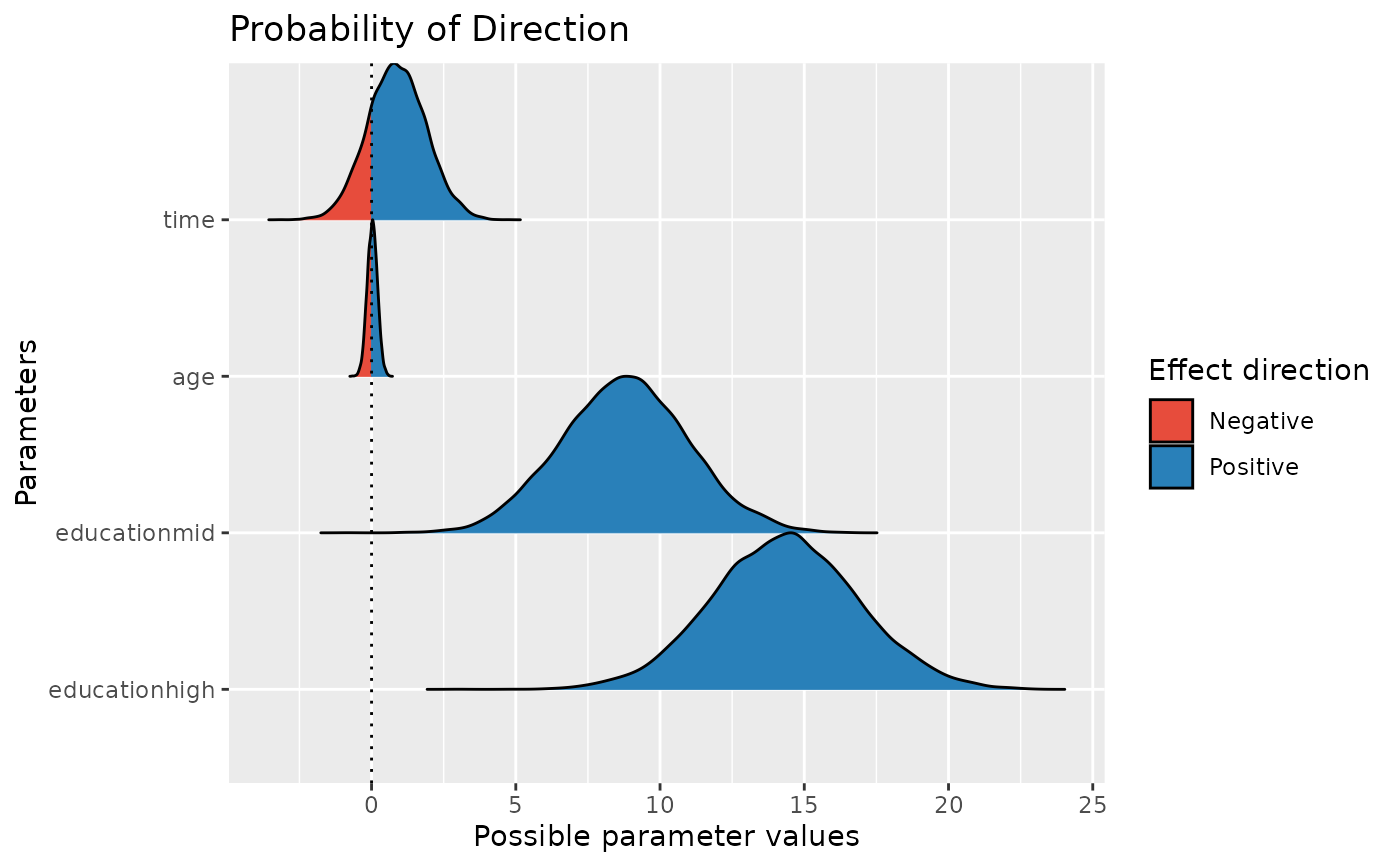
result <- p_direction(model)
plot(result)