This vignette can be referred to by citing the package:
citation("see")
#> To cite package 'see' in publications use:
#>
#>   Lüdecke et al., (2021). see: An R Package for Visualizing Statistical
#>   Models. Journal of Open Source Software, 6(64), 3393.
#>   https://doi.org/10.21105/joss.03393
#>
#> A BibTeX entry for LaTeX users is
#>
#>   @Article{,
#>     title = {{see}: An {R} Package for Visualizing Statistical Models},
#>     author = {Daniel Lüdecke and Indrajeet Patil and Mattan S. Ben-Shachar and Brenton M. Wiernik and Philip Waggoner and Dominique Makowski},
#>     journal = {Journal of Open Source Software},
#>     year = {2021},
#>     volume = {6},
#>     number = {64},
#>     pages = {3393},
#>     doi = {10.21105/joss.03393},
#>   }
Introduction
parameters’ primary goal is to provide utilities for processing the parameters of various statistical models (see here for a list of supported models). Beyond computing p-values, CIs, Bayesian indices and other measures for a wide variety of models, this package implements features like bootstrapping of parameters and models, feature reduction (feature extraction and variable selection), or tools for data reduction like functions to perform cluster, factor or principal component analysis.
Another important goal of the parameters package is to facilitate and streamline the process of reporting results of statistical models, which includes the easy and intuitive calculation of standardized estimates or robust standard errors and p-values. parameters therefor offers a simple and unified syntax to process a large variety of (model) objects from many different packages.
For more, see: https://easystats.github.io/parameters/
Setup and Model Fitting
library(parameters)
library(effectsize)
library(insight)
library(see)
library(glmmTMB)
library(lme4)
library(lavaan)
library(metafor)
library(ggplot2)
data("Salamanders")
data("iris")
data("sleepstudy")
data("qol_cancer")

set.seed(12345)
sleepstudy$grp <- sample.int(5, size = 180, replace = TRUE)

theme_set(theme_modern())
# fit three example model
model1 <- glmmTMB(
  count ~ spp + mined + (1 | site),
  ziformula = ~mined,
  family = poisson(),
  data = Salamanders
)
model_parameters(model1, effects = "fixed")
#> # Fixed Effects
#>
#> Parameter   | Log-Mean |   SE |         95% CI |     z |      p
#> ---------------------------------------------------------------
#> (Intercept) |    -0.36 | 0.28 | [-0.90,  0.18] | -1.30 | 0.194
#> spp [PR]    |    -1.27 | 0.24 | [-1.74, -0.80] | -5.27 | < .001
#> spp [DM]    |     0.27 | 0.14 | [ 0.00,  0.54] |  1.95 | 0.051
#> spp [EC-A]  |    -0.57 | 0.21 | [-0.97, -0.16] | -2.75 | 0.006
#> spp [EC-L]  |     0.67 | 0.13 | [ 0.41,  0.92] |  5.20 | < .001
#> spp [DES-L] |     0.63 | 0.13 | [ 0.38,  0.87] |  4.96 | < .001
#> spp [DF]    |     0.12 | 0.15 | [-0.17,  0.40] |  0.78 | 0.435
#> mined [no]  |     1.27 | 0.27 | [ 0.74,  1.80] |  4.72 | < .001
#>
#> # Zero-Inflation
#>
#> Parameter   | Log-Odds |   SE |         95% CI |     z |      p
#> ---------------------------------------------------------------
#> (Intercept) |     0.79 | 0.27 | [ 0.26,  1.32] |  2.90 | 0.004
#> mined [no]  |    -1.84 | 0.31 | [-2.46, -1.23] | -5.87 | < .001


model2 <- lm(Sepal.Length ~ Species * splines::bs(Petal.Width, degree = 2), data = iris)
model_parameters(model2, effects = "fixed")
#> Parameter                | Coefficient |    SE |          95% CI | t(141) |      p
#> ----------------------------------------------------------------------------------
#> (Intercept)              |        4.79 |  0.17 | [  4.45,  5.13] |  27.66 | < .001
#> Species [versicolor]     |       -3.73 |  2.14 | [ -7.96,  0.50] |  -1.74 | 0.083
#> Species [virginica]      |       -2.67 |  2.88 | [ -8.36,  3.03] |  -0.93 | 0.356
#> Petal Width [1st degree] |        2.53 |  2.36 | [ -2.13,  7.20] |   1.07 | 0.285
#> Petal Width [2nd degree] |      -11.18 | 21.14 | [-52.98, 30.62] |  -0.53 | 0.598
#> Petal Width [1st degree] |        5.48 |  4.84 | [ -4.09, 15.05] |   1.13 | 0.260
#> Petal Width [1st degree] |        2.37 |  4.35 | [ -6.22, 10.96] |   0.54 | 0.587
#> Petal Width [2nd degree] |       14.84 | 21.16 | [-26.99, 56.68] |   0.70 | 0.484
#> Petal Width [2nd degree] |       15.81 | 21.32 | [-26.35, 57.96] |   0.74 | 0.460


model3 <- lmer(
  Reaction ~ Days + (1 | grp) + (1 | Subject),
  data = sleepstudy
)

model4 <- lm(QoL ~ time + age + education, data = qol_cancer)
Model Parameters
(related function documentation)
The plot()-method for model_parameters()
creates a so called “forest plot”. In case of models with multiple
components, parameters are separated into facets by model component.
result <- model_parameters(model1, effects = "fixed")

plot(result)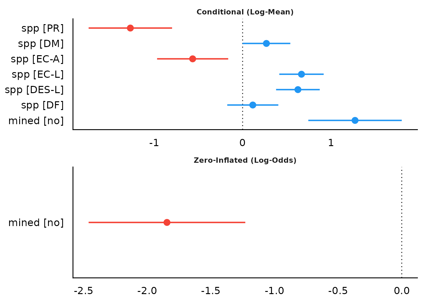
When show_labels is TRUE, coefficients and
confidence intervals are added to the plot. Adjust the text size with
size_text.
plot(result, show_labels = TRUE, size_text = 4)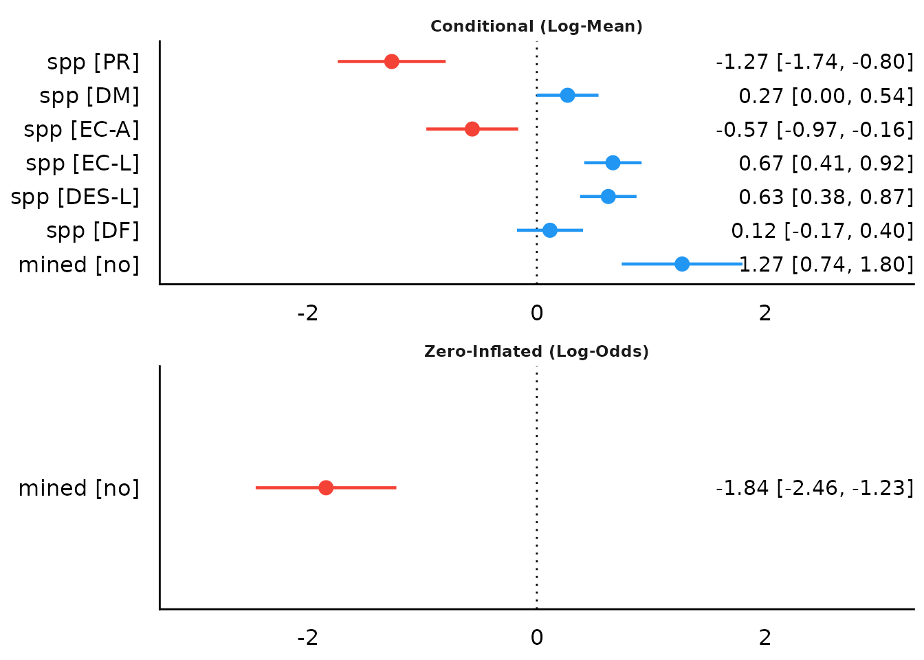
This also works for exponentiated coefficients.
result <- model_parameters(model1, exponentiate = TRUE, effects = "fixed")
plot(result, show_labels = TRUE, size_text = 4)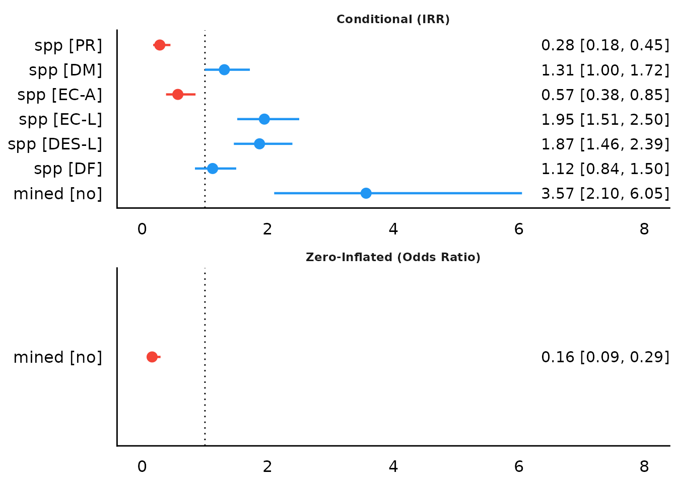
It is also possible to plot only the count-model component. This is
done in model_parameters() via the component
argument. In easystats-functions, the count-component has the more
generic name "conditional".
result <- model_parameters(model1, exponentiate = TRUE, component = "conditional")
plot(result)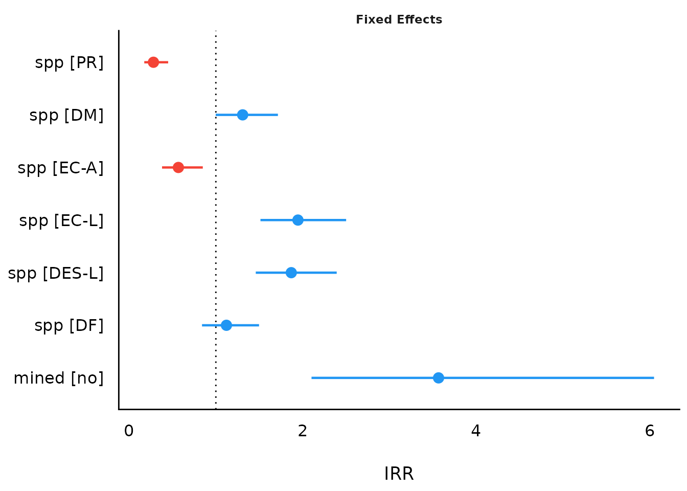
As compared to the classical summary()-output,
model_parameters(), and hence the
plot()-method, tries to create human readable, prettier
parameters names.
result <- model_parameters(model2)

plot(result)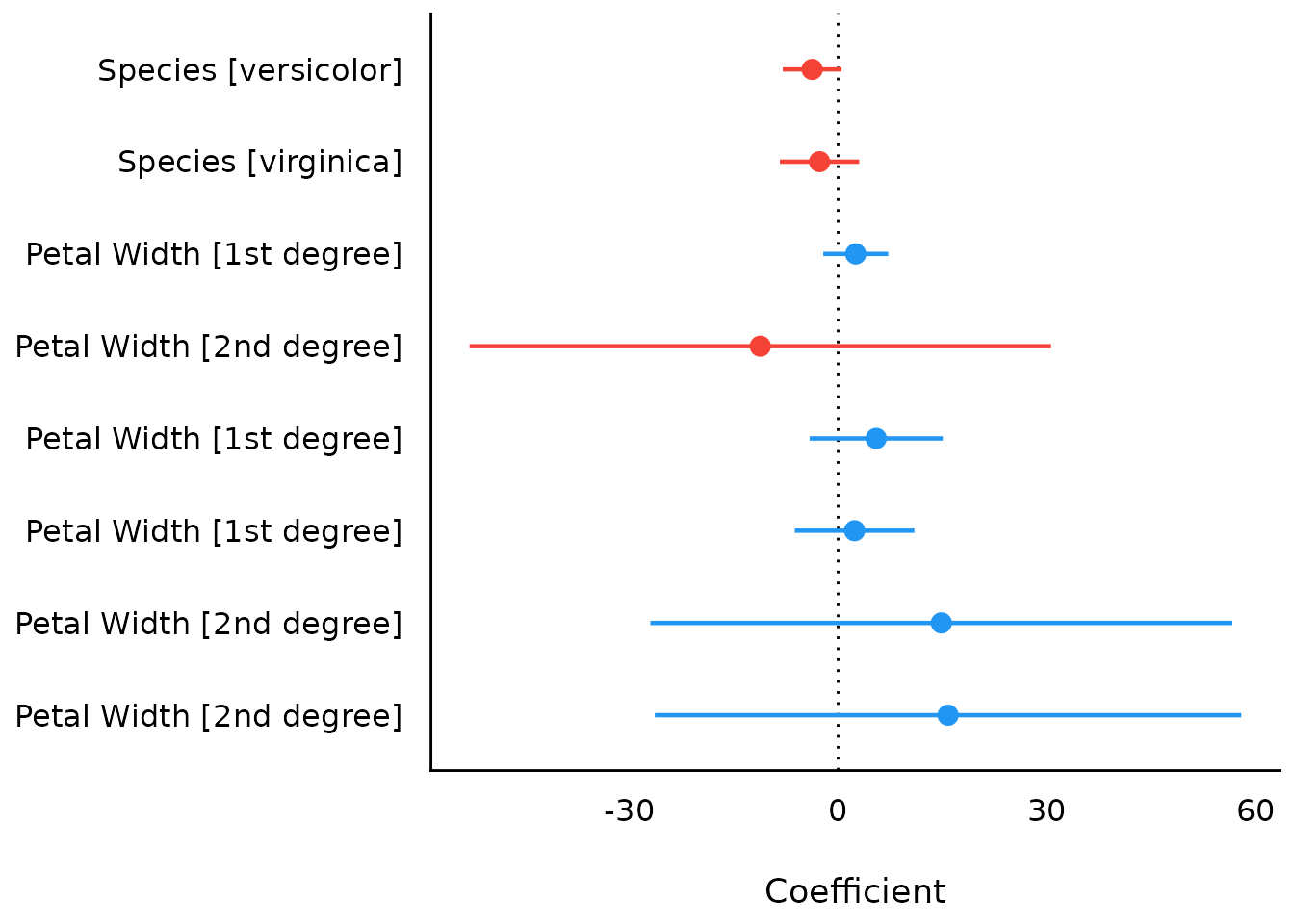
Including group levels of random effects
result <- model_parameters(model3, group_level = TRUE)
plot(result)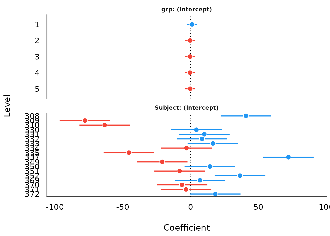
Changing parameter names in the plot
By default, model_parameters() returns a data frame,
where the parameter names are found in the column
Parameter. These names are used by default in the generated
plot:
plot(model_parameters(model4))
However, there are several ways to change the the names of the
parameters. Since plot() returns ggplot objects,
these can be easily modified, e.g. by adding a
scale_y_discrete() layer. Note the correct order of the
labels!
library(ggplot2)
plot(model_parameters(model4)) +
  scale_y_discrete(
    labels = c("Eucation (high-level)", "Education (mid-level)", "Age", "Time")
  )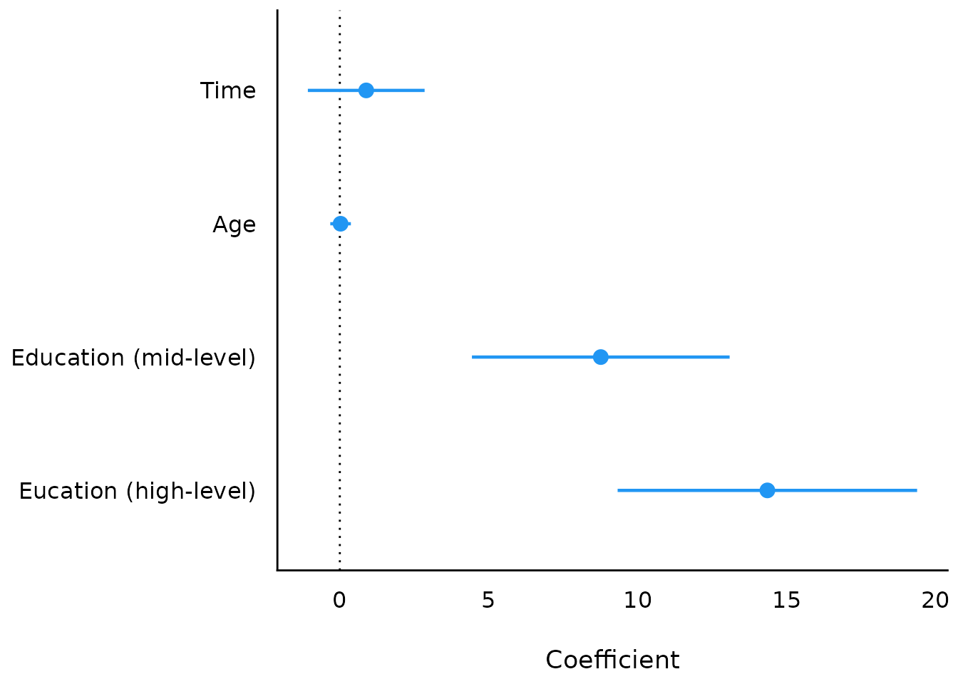
Another way would be changing the values of the
Parameter column before calling plot():
mp <- model_parameters(model4)
mp$Parameter <- c(
  "(Intercept)", "Time", "Age", "Education (mid-level)",
  "Eucation (high-level)"
)
plot(mp)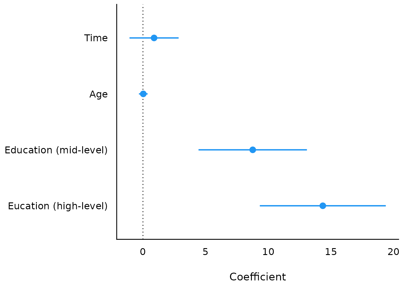
Simulated Model Parameters
simulate_parameters() computes simulated draws of
parameters and their related indices such as Confidence Intervals (CI)
and p-values. Simulating parameter draws can be seen as a
(computationally faster) alternative to bootstrapping.
As simulate_parameters() is based on
simulate_model() and thus simulates many draws for each
parameter, plot() will produce similar plots as the density
estimation plots from
Bayesian models.
result <<- simulate_parameters(model1)

plot(result)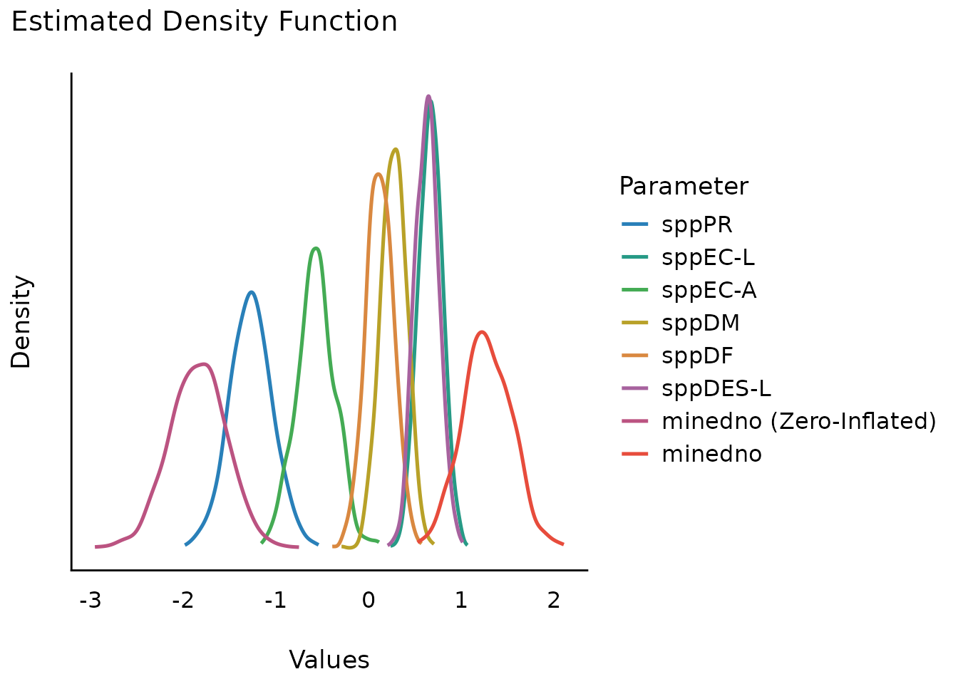
plot(result, stack = FALSE)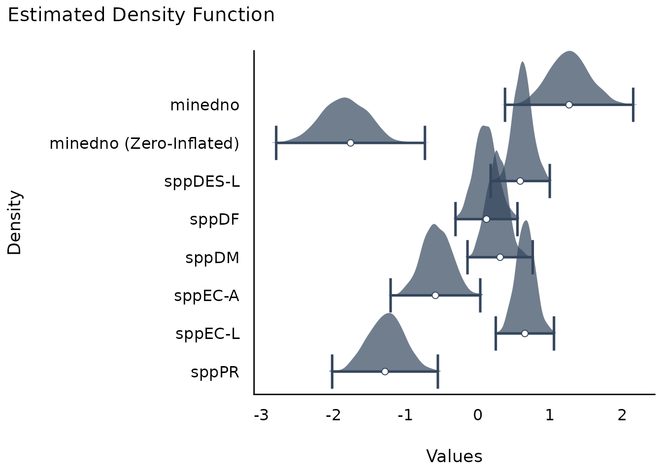
To avoid vertical overlapping, use normalize_height.
plot(result, stack = FALSE, normalize_height = TRUE)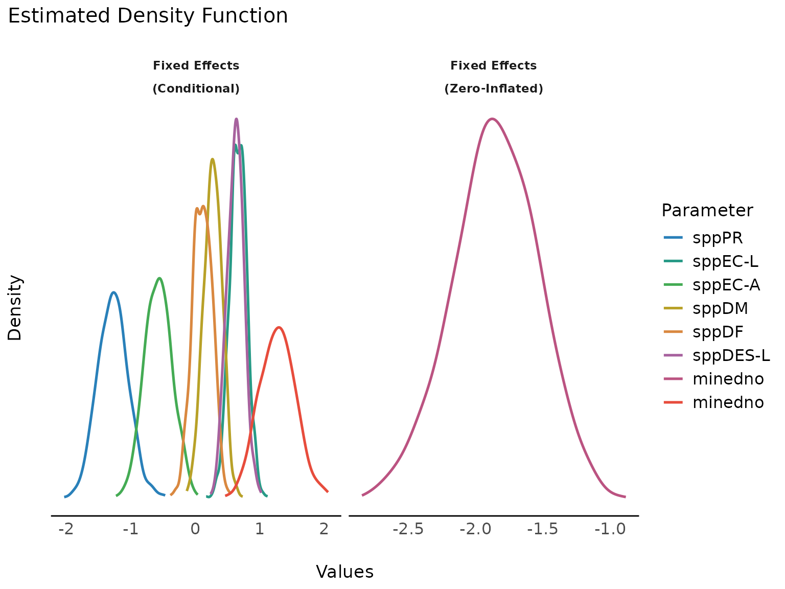
plot(result, n_columns = 2)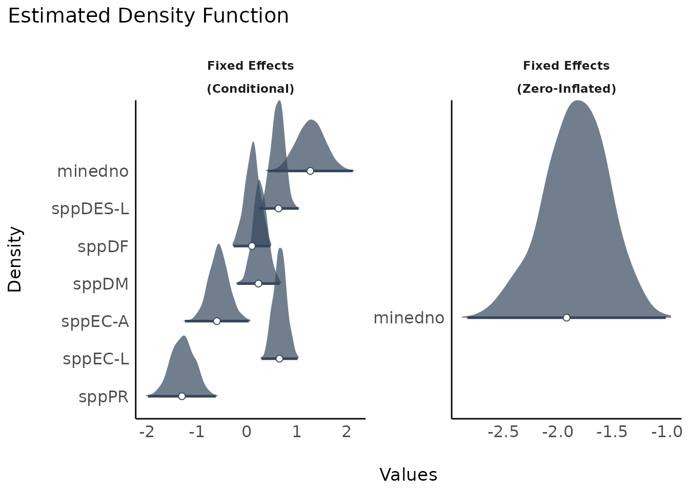
plot(result, n_columns = 2, stack = FALSE)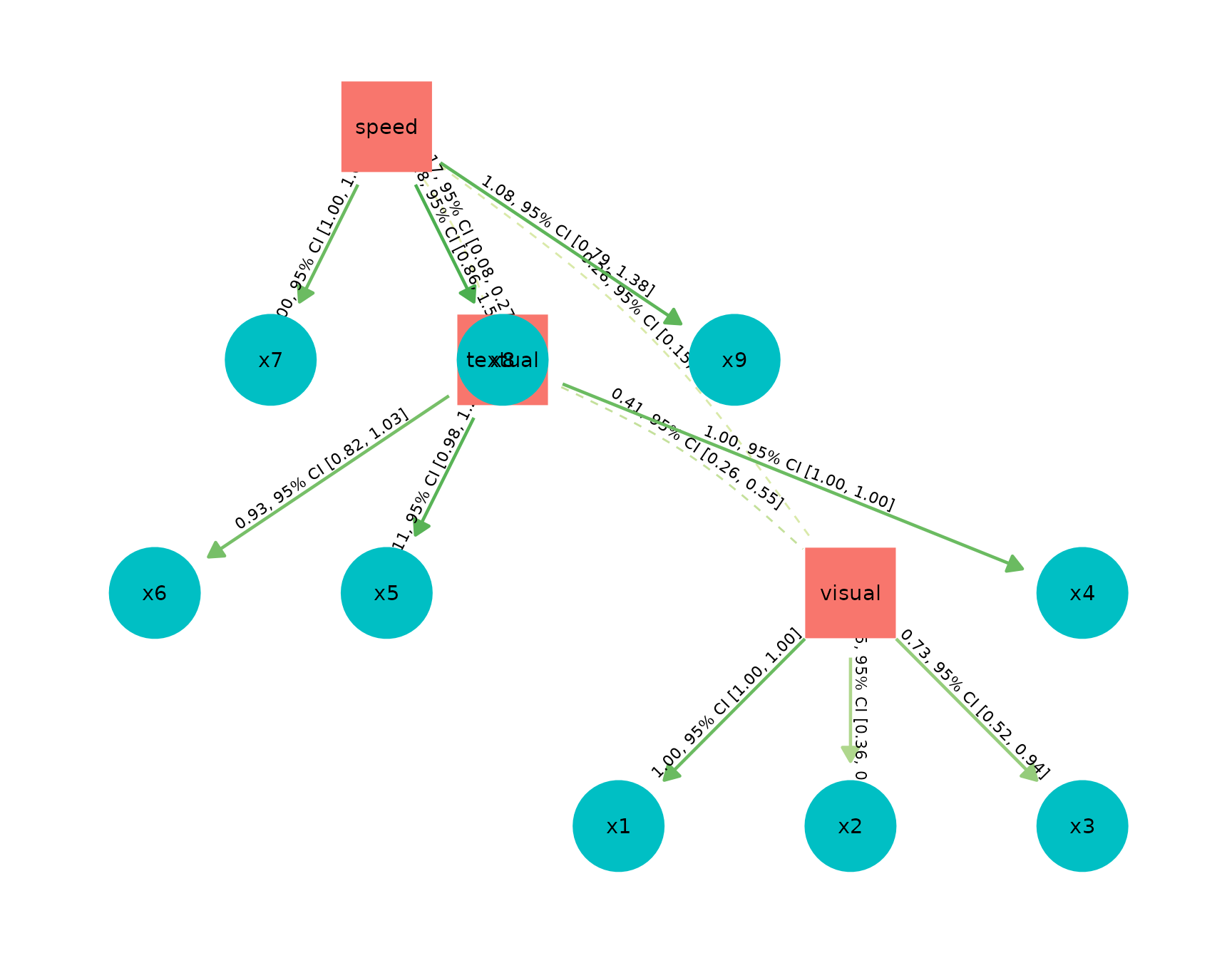
Model Parameters of SEM models
structure <- " visual  =~ x1 + x2 + x3
               textual =~ x4 + x5 + x6
               speed   =~ x7 + x8 + x9 "

model <- lavaan::cfa(structure, data = HolzingerSwineford1939)
result <- model_parameters(model)
plot(result)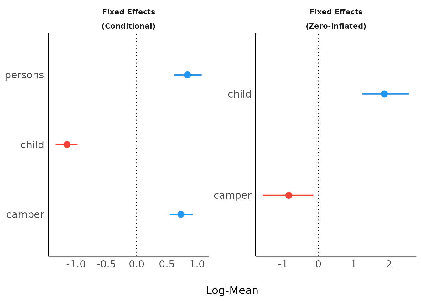
Model Parameters of Bayesian models
model_parameters() for Bayesian models will produce
“forest plots” (instead of density
estimations).
# We download the model to save computation time. Here is the code
# to refit the exact model used below...

# zinb <- read.csv("http://stats.idre.ucla.edu/stat/data/fish.csv")
# set.seed(123)
# model <- brm(bf(
#     count ~ persons + child + camper + (1 | persons),
#     zi ~ child + camper + (1 | persons)
#   ),
#   data = zinb,
#   family = zero_inflated_poisson()
# )
brms_model <- insight::download_model("brms_zi_2")
result <- model_parameters(
  brms_model,
  effects = "all",
  component = "all",
  verbose = FALSE
)

plot(result)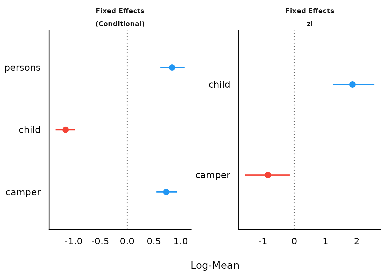
Including group levels of random effects
result <- model_parameters(brms_model,
  effects = "all",
  component = "all",
  group_level = TRUE,
  verbose = FALSE
)
plot(result)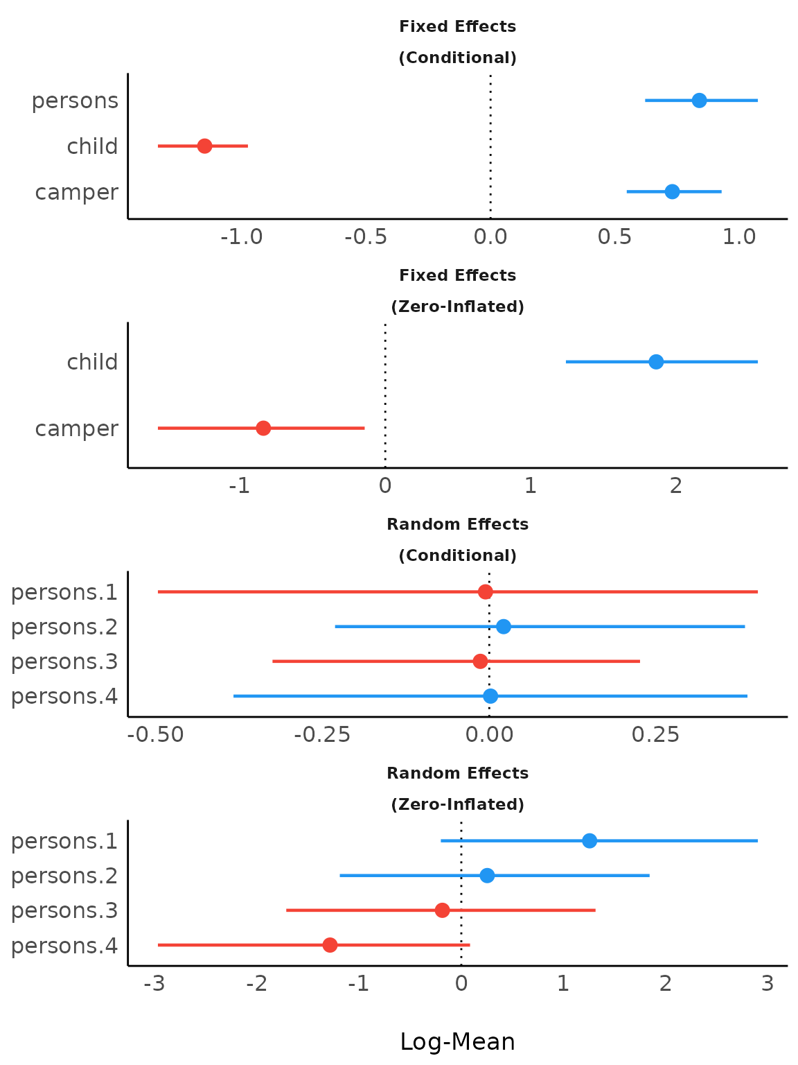
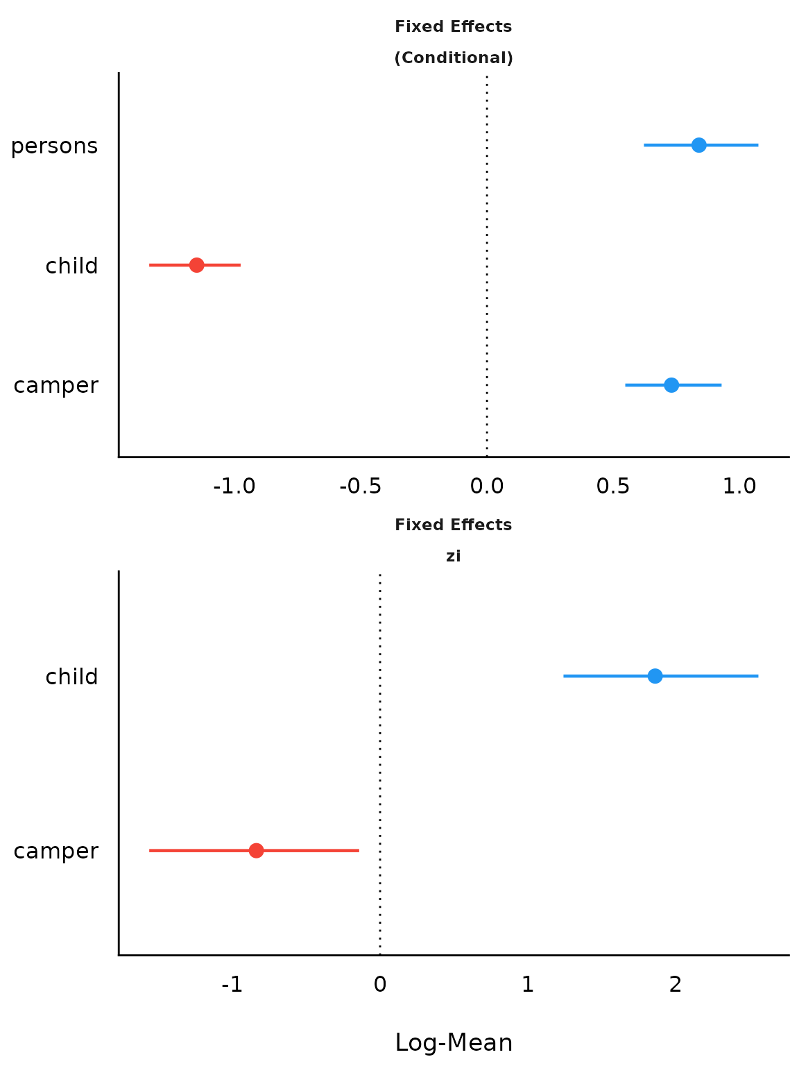
Including Intercepts and Variance Estimates for Random Intercepts
plot(result, show_intercept = TRUE)
Model Parameters of Meta-Analysis models
mydat <<- data.frame(
  effectsize = c(-0.393, 0.675, 0.282, -1.398),
  standarderror = c(0.317, 0.317, 0.13, 0.36)
)

ma <- rma(yi = effectsize, sei = standarderror, method = "REML", data = mydat)
result <- model_parameters(ma)

result
#> Meta-analysis using 'metafor'
#>
#> Parameter | Coefficient |   SE |         95% CI |     z |      p | Weight
#> -------------------------------------------------------------------------
#> Study 1   |       -0.39 | 0.32 | [-1.01,  0.23] | -1.24 | 0.215  |   9.95
#> Study 2   |        0.68 | 0.32 | [ 0.05,  1.30] |  2.13 | 0.033  |   9.95
#> Study 3   |        0.28 | 0.13 | [ 0.03,  0.54] |  2.17 | 0.030  |  59.17
#> Study 4   |       -1.40 | 0.36 | [-2.10, -0.69] | -3.88 | < .001 |   7.72
#> Overall   |       -0.18 | 0.44 | [-1.05,  0.68] | -0.42 | 0.676  |
plot(result)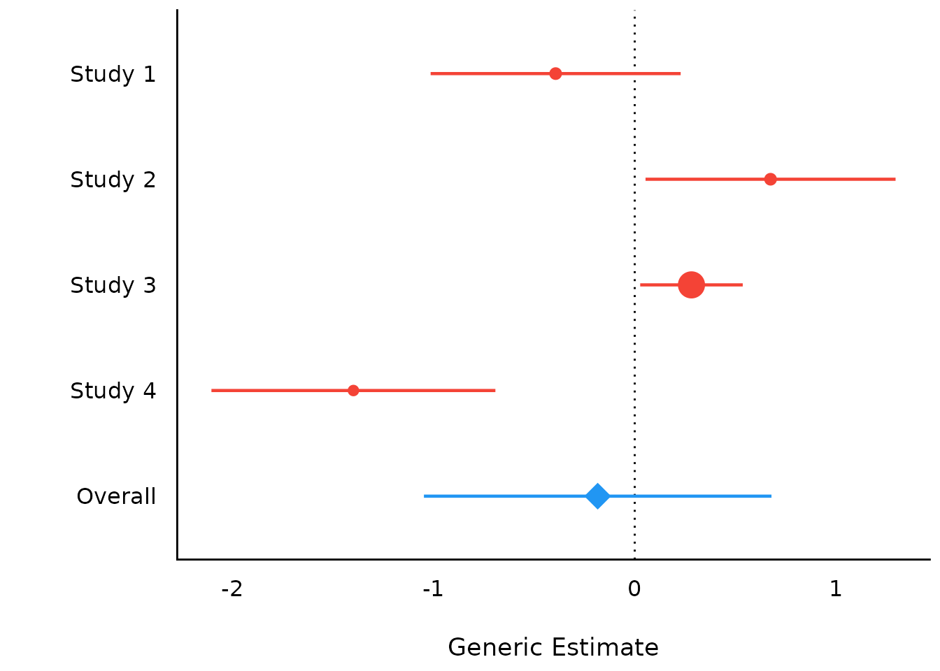
If show_labels is TRUE, estimates and
confidence intervals are included in the plot. Adjust the text size with
size_text.
plot(result, show_labels = TRUE, size_text = 4)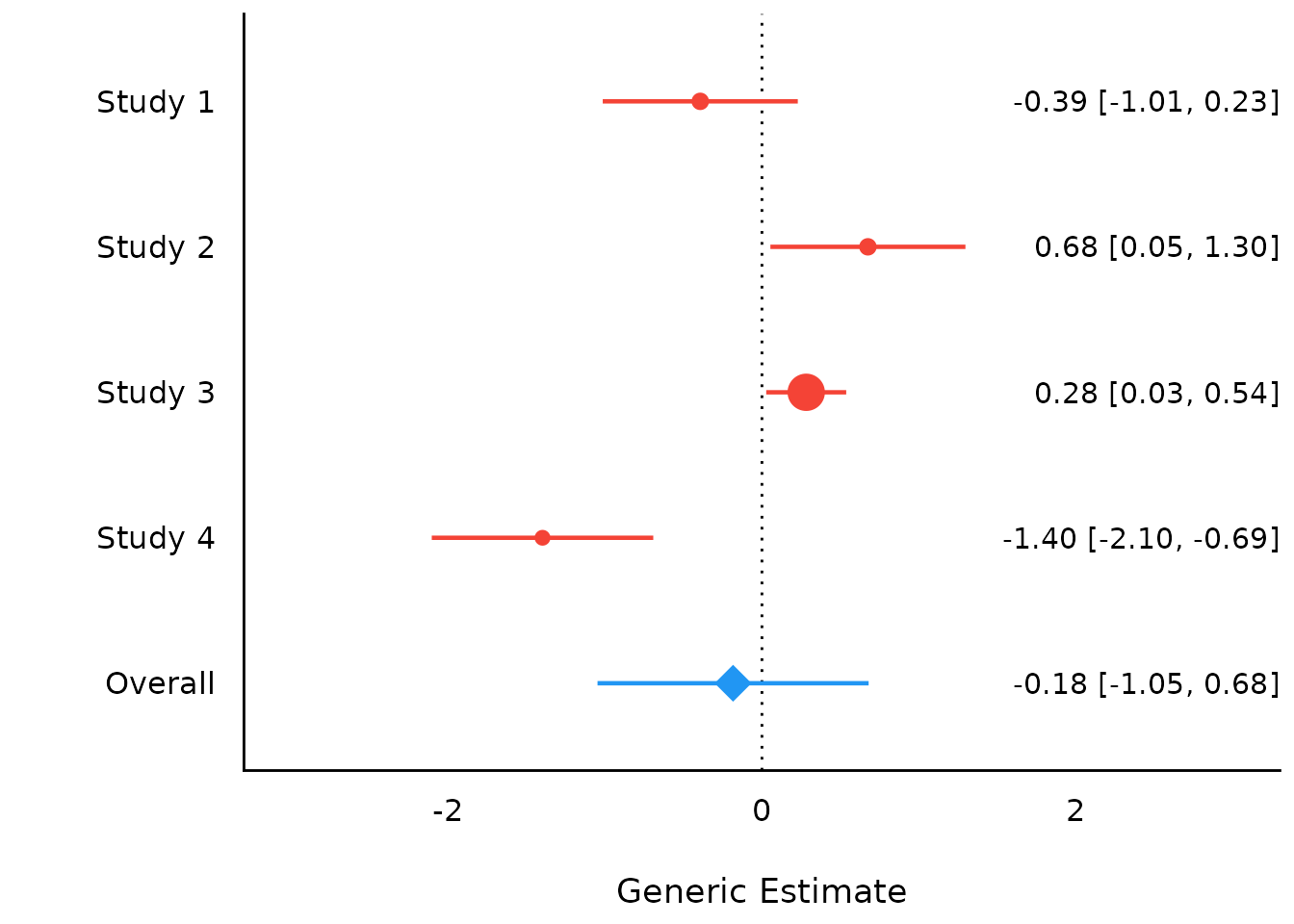

Model Parameters of Meta-Analysis Models with Subgroups
set.seed(123)
data(dat.bcg)
dat <- escalc(
  measure = "RR",
  ai = tpos,
  bi = tneg,
  ci = cpos,
  di = cneg,
  data = dat.bcg
)
dat$author <- make.unique(dat$author)
dat$disease <- sample(c("Cancer", "CVD", "Depression"), size = nrow(dat), replace = TRUE)
mydat <<- dat
model <- rma(yi, vi, mods = ~disease, data = mydat, digits = 3, slab = author)
result <- model_parameters(model)

result
#> # Depression
#>
#> Parameter            | Coefficient |   SE |         95% CI |     z |      p | Weight
#> ------------------------------------------------------------------------------------
#> Aronson              |       -0.89 | 0.57 | [-2.01,  0.23] | -1.56 | 0.119  |   3.07
#> Ferguson & Simes     |       -1.59 | 0.44 | [-2.45, -0.72] | -3.59 | < .001 |   5.14
#> Rosenthal et al      |       -1.35 | 0.64 | [-2.61, -0.08] | -2.09 | 0.036  |   2.41
#> Frimodt-Moller et al |       -0.22 | 0.23 | [-0.66,  0.23] | -0.96 | 0.336  |  19.53
#> Coetzee & Berjak     |       -0.47 | 0.24 | [-0.94,  0.00] | -1.98 | 0.048  |  17.72
#> Overall              |       -0.12 | 0.59 | [-1.28,  1.04] | -0.20 | 0.841  |
#>
#> # CVD
#>
#> Parameter          | Coefficient |   SE |         95% CI |      z |      p | Weight
#> -----------------------------------------------------------------------------------
#> Hart & Sutherland  |       -1.44 | 0.14 | [-1.72, -1.16] | -10.19 | < .001 |  49.97
#> Stein & Aronson    |       -0.79 | 0.08 | [-0.95, -0.62] |  -9.46 | < .001 | 144.81
#> Vandiviere et al   |       -1.62 | 0.47 | [-2.55, -0.70] |  -3.43 | < .001 |   4.48
#> TPT Madras         |        0.01 | 0.06 | [-0.11,  0.14] |   0.19 | 0.849  | 252.42
#> Comstock et al     |       -0.34 | 0.11 | [-0.56, -0.12] |  -3.05 | 0.002  |  80.57
#> Comstock & Webster |        0.45 | 0.73 | [-0.98,  1.88] |   0.61 | 0.541  |   1.88
#> Overall            |        0.03 | 0.56 | [-1.08,  1.13] |   0.05 | 0.963  |
#>
#> # Cancer
#>
#> Parameter         | Coefficient |   SE |         95% CI |     z |      p | Weight
#> ---------------------------------------------------------------------------------
#> Rosenthal et al.1 |       -1.37 | 0.27 | [-1.90, -0.84] | -5.07 | < .001 |  13.69
#> Comstock et al.1  |       -0.02 | 0.27 | [-0.54,  0.51] | -0.06 | 0.948  |  14.00
#> Overall           |       -0.69 | 0.49 | [-1.65,  0.26] | -1.42 | 0.155  |
plot(result)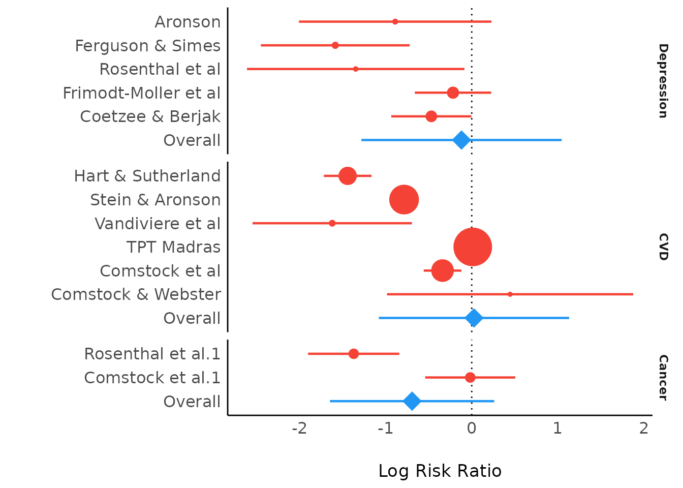
Bayesian Meta-Analysis using brms
We download the model to save computation time, but here is the code to refit the exact model used below:
# Data from
# https://github.com/MathiasHarrer/Doing-Meta-Analysis-in-R/blob/master/_data/Meta_Analysis_Data.RData
set.seed(123)
priors <- c(
  prior(normal(0, 1), class = Intercept),
  prior(cauchy(0, 0.5), class = sd)
)

model <- brm(
  TE | se(seTE) ~ 1 + (1 | Author),
  data = Meta_Analysis_Data,
  prior = priors,
  iter = 4000
)
library(brms)
model <- insight::download_model("brms_meta_1")
result <- model_parameters(model)

result
#> # Studies
#>
#> Parameter              | Median |        95% CI | Weight |     pd |  Rhat | ESS (tail)
#> --------------------------------------------------------------------------------------
#> Overall                |   0.57 | [ 0.40, 0.76] |        |   100% | 1.000 |       4648
#> Call et al             |   0.63 | [ 0.28, 1.03] |   3.83 | 99.95% |       |
#> Cavanagh et al         |   0.43 | [ 0.10, 0.75] |   5.09 | 99.45% |       |
#> DanitzOrsillo          |   1.05 | [ 0.54, 1.67] |   2.89 |   100% |       |
#> de Vibe et al          |   0.25 | [ 0.02, 0.47] |   8.49 | 98.39% |       |
#> Frazier et al          |   0.45 | [ 0.20, 0.71] |   6.91 | 99.91% |       |
#> Frogeli et al          |   0.60 | [ 0.30, 0.93] |   5.10 | 99.99% |       |
#> Gallego et al          |   0.65 | [ 0.31, 1.03] |   4.45 |   100% |       |
#> Hazlett-Stevens & Oren |   0.54 | [ 0.20, 0.88] |   4.75 | 99.85% |       |
#> Hintz et al            |   0.36 | [ 0.08, 0.64] |   5.95 | 99.36% |       |
#> Kang et al             |   0.84 | [ 0.41, 1.40] |   2.97 |   100% |       |
#> Kuhlmann et al         |   0.27 | [-0.09, 0.57] |   5.14 | 93.21% |       |
#> Lever Taylor et al     |   0.46 | [ 0.10, 0.81] |   4.33 | 99.34% |       |
#> Phang et al            |   0.55 | [ 0.19, 0.92] |   4.09 | 99.83% |       |
#> Rasanen et al          |   0.49 | [ 0.10, 0.87] |   3.88 | 99.26% |       |
#> Ratanasiripong         |   0.54 | [ 0.09, 0.99] |   2.85 | 99.01% |       |
#> Shapiro et al          |   0.96 | [ 0.50, 1.53] |   3.17 |   100% |       |
#> SongLindquist          |   0.59 | [ 0.25, 0.95] |   4.41 | 99.95% |       |
#> Warnecke et al         |   0.58 | [ 0.21, 0.96] |   4.02 | 99.81% |       |
#>
#> # Tau
#>
#> Parameter | Median |       95% CI |   pd
#> ----------------------------------------
#> tau       |   0.29 | [0.12, 0.51] | 100%
plot(result)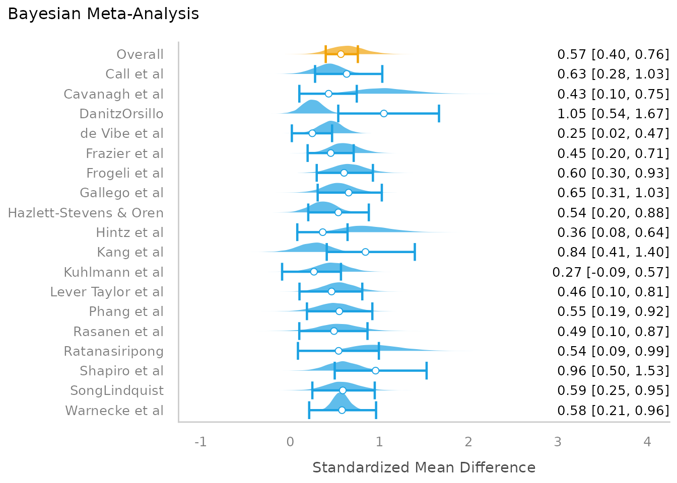
Comparison of Models
(related function documentation)
data(iris)
# shorter variable name
iris$Length <- iris$Petal.Length
lm1 <- lm(Sepal.Length ~ Species, data = iris)
lm2 <- lm(Sepal.Length ~ Species + Length, data = iris)
lm3 <- lm(Sepal.Length ~ Species * Length, data = iris)

result <- compare_parameters(lm1, lm2, lm3)
plot(result)

Equivalence Testing
(related function documentation)
For fixed effects
# default rules, like in bayestestR::equivalence_test()
result <- equivalence_test(model4)
result
#> # TOST-test for Practical Equivalence
#>
#>   ROPE: [-1.99 1.99]
#>
#> Parameter        |         90% CI |   SGPV | Equivalence |      p
#> -----------------------------------------------------------------
#> (Intercept)      | [59.33, 68.41] | < .001 |    Rejected | > .999
#> time             | [-0.76,  2.53] | 0.905  |   Undecided | 0.137
#> age              | [-0.26,  0.32] | > .999 |    Accepted | < .001
#> education [mid]  | [ 5.13, 12.39] | < .001 |    Rejected | 0.999
#> education [high] | [10.14, 18.57] | < .001 |    Rejected | > .999

plot(result)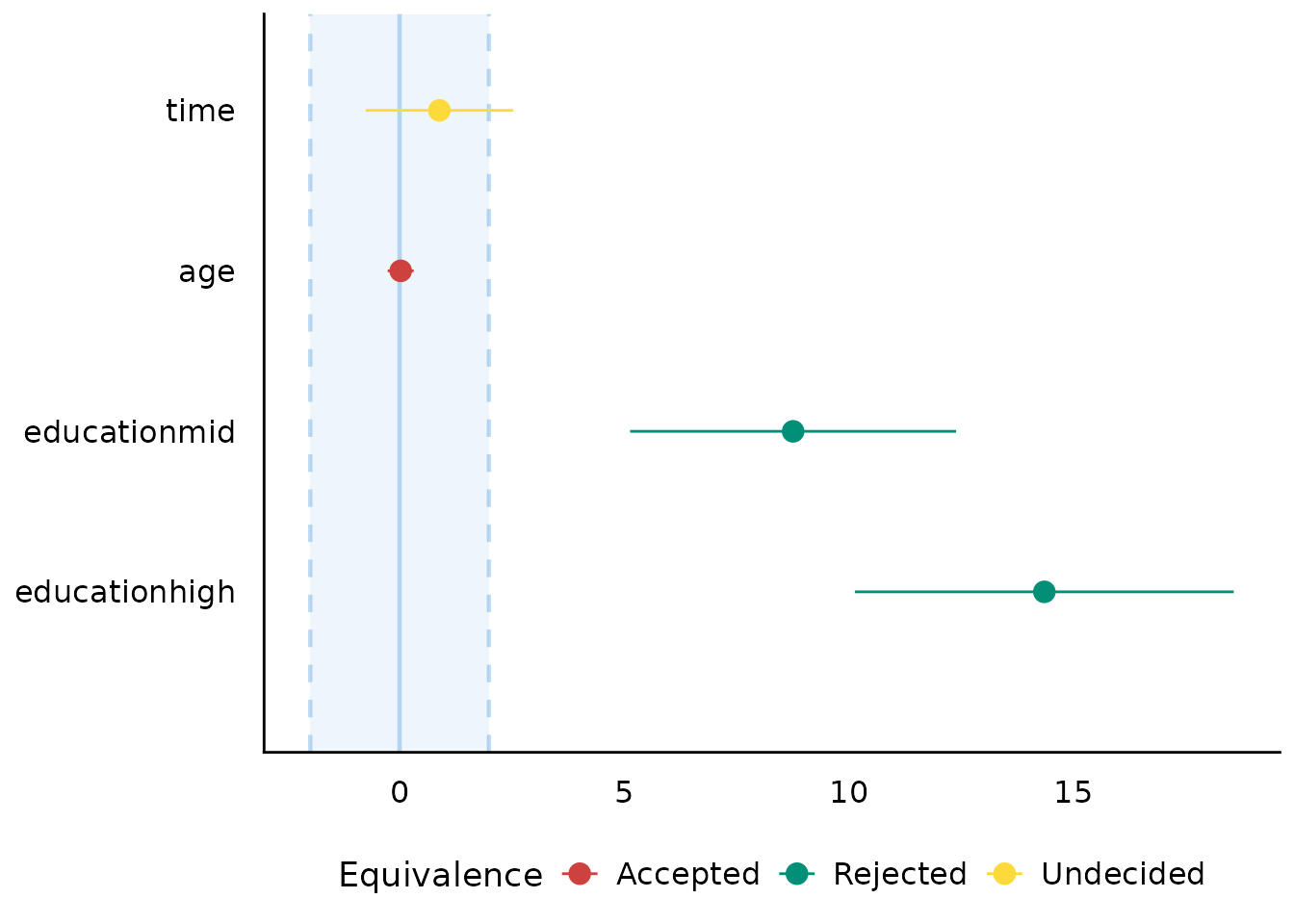
result <- equivalence_test(model4, rule = "cet")
result
#> # Conditional Equivalence Testing
#>
#>   ROPE: [-1.99 1.99]
#>
#> Parameter        |         90% CI |   SGPV | Equivalence |      p
#> -----------------------------------------------------------------
#> (Intercept)      | [59.33, 68.41] | < .001 |    Rejected | > .999
#> time             | [-0.76,  2.53] | 0.905  |   Undecided | 0.137
#> age              | [-0.26,  0.32] | > .999 |    Accepted | < .001
#> education [mid]  | [ 5.13, 12.39] | < .001 |    Rejected | 0.999
#> education [high] | [10.14, 18.57] | < .001 |    Rejected | > .999

plot(result)
For random effects
result <- equivalence_test(model3, effects = "random")
result
#> # TOST-test for Practical Equivalence
#>
#>   ROPE: [-5.63 5.63]
#>
#> Group: grp
#>
#> Parameter | Estimate | Group |           90% CI |   SGPV | Equivalence
#> ----------------------------------------------------------------------
#> 1         |     1.18 |   grp | [ -1.91,   4.28] | 0.998  |    Accepted
#> 2         |    -0.21 |   grp | [ -3.27,   2.84] | > .999 |    Accepted
#> 3         |    -0.25 |   grp | [ -3.33,   2.83] | > .999 |    Accepted
#> 4         |    -0.48 |   grp | [ -3.56,   2.60] | > .999 |    Accepted
#> 5         |    -0.24 |   grp | [ -3.33,   2.85] | > .999 |    Accepted
#> Group: Subject
#>
#> Parameter | Estimate |   Group |           90% CI |   SGPV | Equivalence
#> ------------------------------------------------------------------------
#> 308       |    40.86 | Subject | [ 25.22,  56.50] | < .001 |    Rejected
#> 309       |   -77.88 | Subject | [-93.51, -62.24] | < .001 |    Rejected
#> 310       |   -63.28 | Subject | [-78.91, -47.65] | < .001 |    Rejected
#> 330       |     4.32 | Subject | [-11.32,  19.96] | 0.459  |   Undecided
#> 331       |    10.18 | Subject | [ -5.45,  25.80] | 0.261  |   Undecided
#> 332       |     8.47 | Subject | [ -7.17,  24.10] | 0.323  |   Undecided
#> 333       |    16.44 | Subject | [  0.81,  32.07] | 0.085  |    Rejected
#> 334       |    -3.00 | Subject | [-18.65,  12.65] | 0.489  |   Undecided
#> 335       |   -45.48 | Subject | [-61.11, -29.85] | < .001 |    Rejected
#> 337       |    72.16 | Subject | [ 56.54,  87.79] | < .001 |    Rejected
#> 349       |   -20.91 | Subject | [-36.57,  -5.25] | 0.028  |    Rejected
#> 350       |    14.23 | Subject | [ -1.41,  29.88] | 0.134  |   Undecided
#> 351       |    -8.07 | Subject | [-23.74,   7.59] | 0.337  |   Undecided
#> 352       |    36.44 | Subject | [ 20.76,  52.12] | < .001 |    Rejected
#> 369       |     6.97 | Subject | [ -8.66,  22.60] | 0.376  |   Undecided
#> 370       |    -6.31 | Subject | [-21.96,   9.34] | 0.399  |   Undecided
#> 371       |    -3.34 | Subject | [-18.96,  12.29] | 0.483  |   Undecided
#> 372       |    18.21 | Subject | [  2.57,  33.84] | 0.056  |    Rejected

plot(result)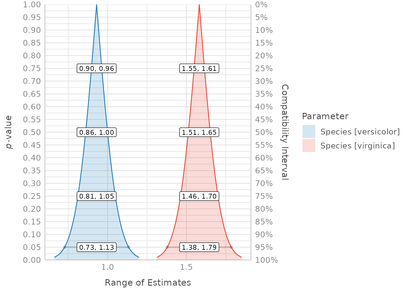
p-value function and consonance/compatibility plot
(related function documentation)
data(iris)
model <- lm(Sepal.Length ~ Species, data = iris)

result <- p_function(model)
plot(result)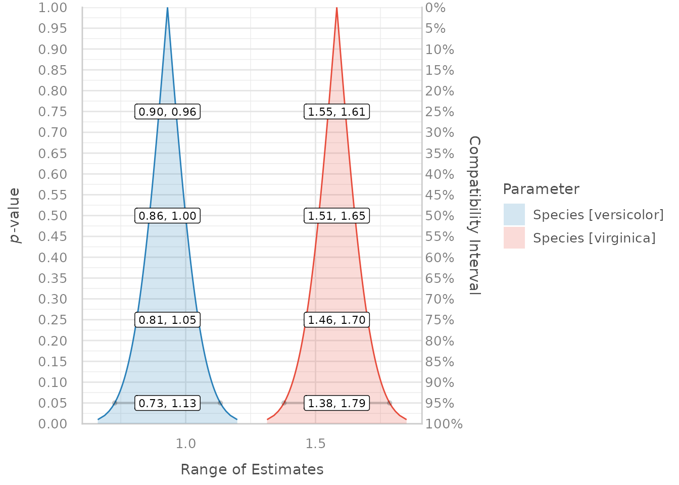
result <- p_function(model, ci_levels = c(0.5, 0.7, emph = 0.9))
plot(result, size_line = c(0.6, 1.2))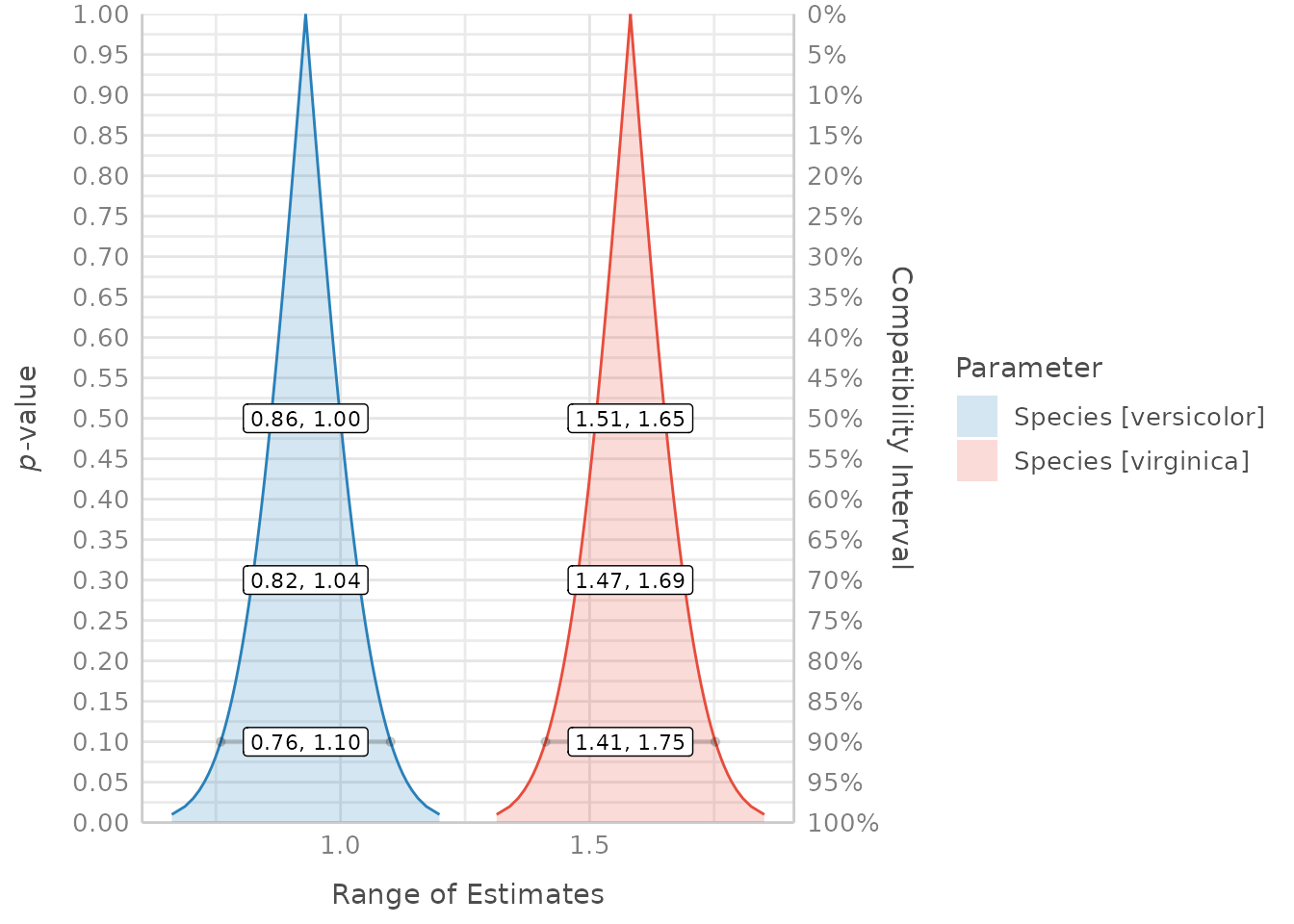
Probability of Direction
(related function documentation)
data(qol_cancer)
model <- lm(QoL ~ time + age + education, data = qol_cancer)
result <- p_direction(model)

plot(result)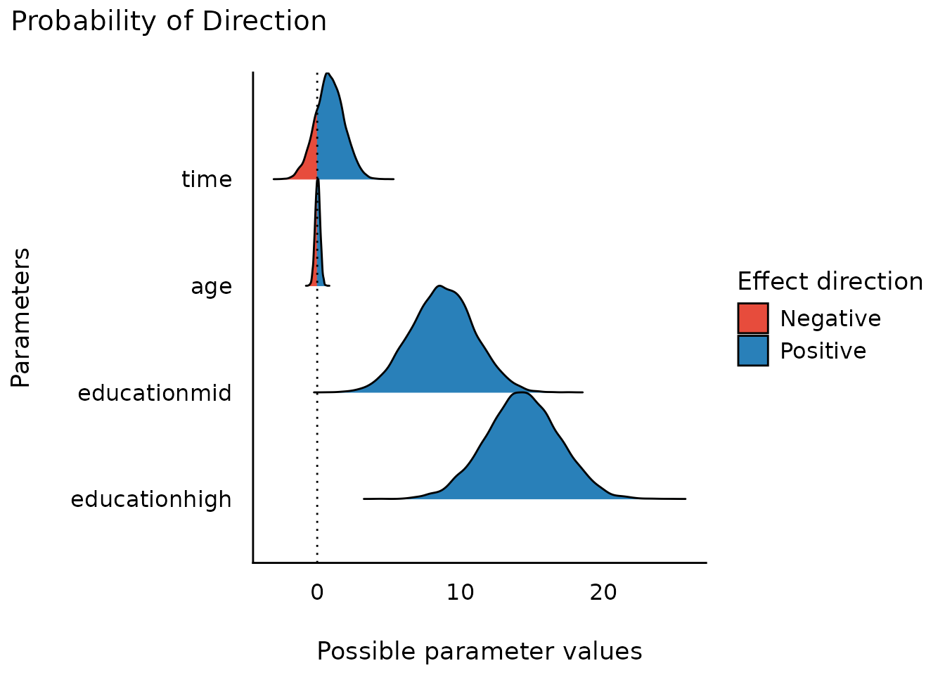
Practical Significance
(related function documentation)
data(qol_cancer)
model <- lm(QoL ~ time + age + education, data = qol_cancer)
result <- p_significance(model)

plot(result)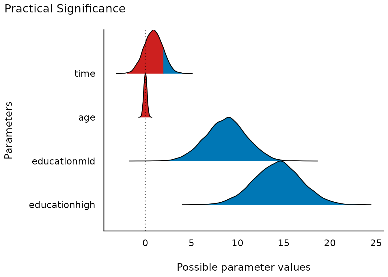
Principal Component Analysis
(related function documentation)
# Bars
data(mtcars)
result <- principal_components(mtcars[, 1:7], n = "all", threshold = 0.2)
result
#> # Loadings from Principal Component Analysis (no rotation)
#>
#> Variable |   PC1 |   PC2 |  PC3 |   PC4 |  PC5 |   PC6 | Complexity
#> -------------------------------------------------------------------
#> mpg      | -0.93 |       |      | -0.30 |      |       |       1.30
#> cyl      |  0.96 |       |      |       |      | -0.21 |       1.18
#> disp     |  0.95 |       |      | -0.23 |      |       |       1.16
#> hp       |  0.87 |  0.36 |      |       | 0.30 |       |       1.64
#> drat     | -0.75 |  0.48 | 0.44 |       |      |       |       2.47
#> wt       |  0.88 | -0.35 | 0.26 |       |      |       |       1.54
#> qsec     | -0.54 | -0.81 |      |       |      |       |       1.96
#>
#> The 6 principal components accounted for 99.30% of the total variance of the original data (PC1 = 72.66%, PC2 = 16.52%, PC3 = 4.93%, PC4 = 2.26%, PC5 = 1.85%, PC6 = 1.08%).

plot(result)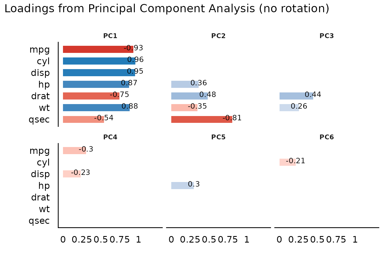
# Graph
result <- principal_components(mtcars[, 1:7], n = 3, rotation = "varimax")
plot(result, type = "graph", arrow_end_gap = 0.15)
# lines
result <- principal_components(
  mtcars[, 1:7],
  n = 3,
  rotation = "varimax",
  threshold = "max",
  sort = TRUE
)

result
#> # Rotated loadings from Principal Component Analysis (varimax-rotation)
#>
#> Variable |   RC1 |   RC2 |   RC3 | Complexity | Uniqueness |  MSA
#> -----------------------------------------------------------------
#> wt       |  0.91 |       |       |       1.31 |       0.03 | 0.77
#> mpg      | -0.82 |       |       |       1.70 |       0.11 | 0.87
#> disp     |  0.79 |       |       |       1.95 |       0.08 | 0.85
#> cyl      |  0.64 |       |       |       2.84 |       0.06 | 0.87
#> qsec     |       | -0.98 |       |       1.02 |       0.03 | 0.61
#> hp       |       |  0.69 |       |       2.09 |       0.09 | 0.90
#> drat     |       |       | -0.90 |       1.43 |       0.01 | 0.85
#>
#> The 3 principal components (varimax rotation) accounted for 94.11% of the total variance of the original data (RC1 = 45.02%, RC2 = 27.79%, RC3 = 21.30%).

plot(result, type = "line", color_text = "white") +
  theme_abyss()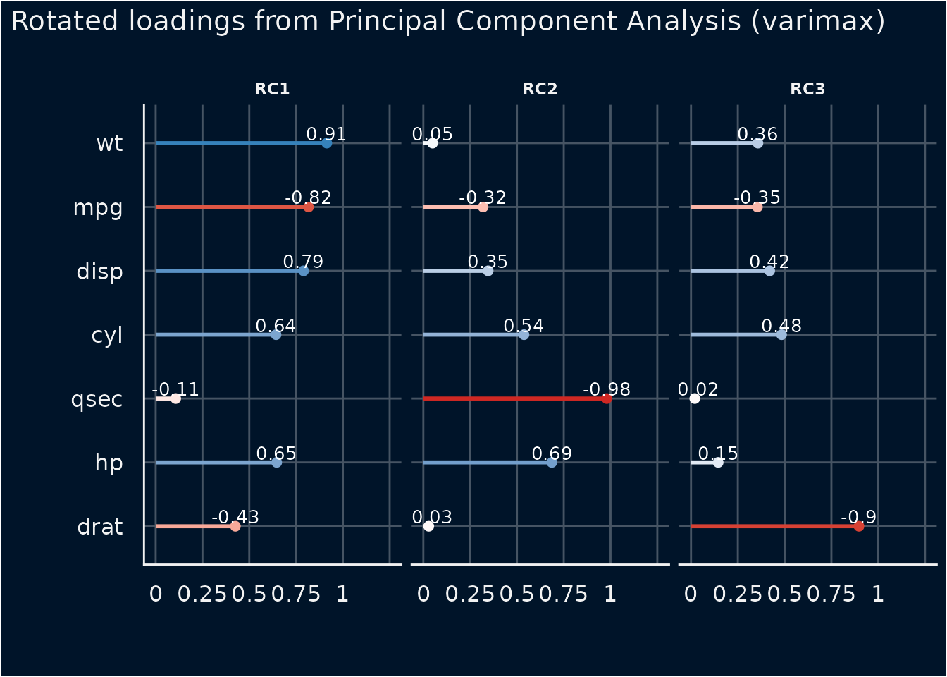
Cluster Analysis
(related function documentation)
Clustering solution
data(iris)
result <- cluster_analysis(iris[, 1:4], n = 3)
result
#> # Clustering Solution
#>
#> The 3 clusters accounted for 76.70% of the total variance of the original data.
#>
#> Cluster | n_Obs | Sum_Squares | Sepal.Length | Sepal.Width | Petal.Length | Petal.Width
#> ---------------------------------------------------------------------------------------
#> 1       |    53 |       44.09 |        -0.05 |       -0.88 |         0.35 |        0.28
#> 2       |    50 |       47.35 |        -1.01 |        0.85 |        -1.30 |       -1.25
#> 3       |    47 |       47.45 |         1.13 |        0.09 |         0.99 |        1.01
#>
#> # Indices of model performance
#>
#> Sum_Squares_Total | Sum_Squares_Between | Sum_Squares_Within |    R2
#> --------------------------------------------------------------------
#> 596               |             457.112 |            138.888 | 0.767
#>
#> # You can access the predicted clusters via `predict()`.
plot(result)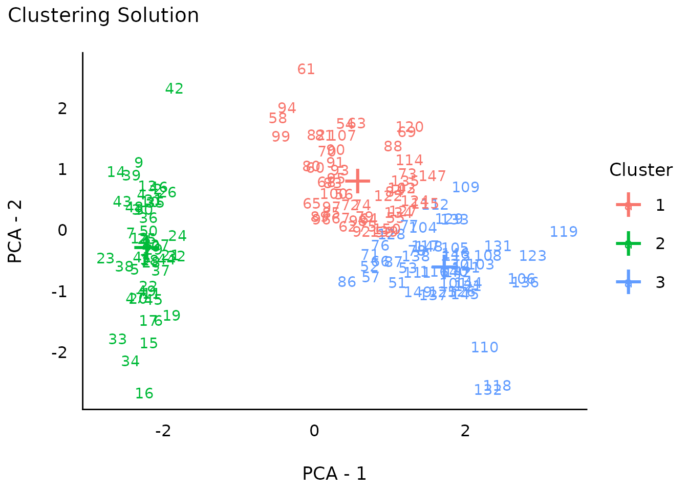
result <- cluster_analysis(iris[, 1:4], n = 4)
plot(result)
Cluster centers
s <- summary(result)
s
#>   Cluster Sepal.Length Sepal.Width Petal.Length Petal.Width
#> 1       1    1.3926646   0.2323817   1.15674505  1.21327591
#> 2       2   -0.9987207   0.9032290  -1.29875725 -1.25214931
#> 3       3   -0.4201099  -1.4246794   0.03924137 -0.05279511
#> 4       4    0.3558492  -0.3930869   0.58460377  0.54663615

plot(s)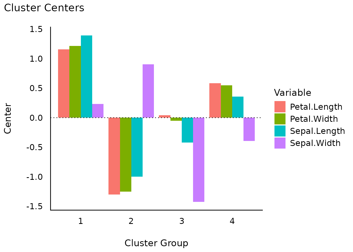
Number of Components/Factors to Retain
(related function documentation)
data(mtcars)
result <- n_factors(mtcars, type = "PCA")
result
#> # Method Agreement Procedure:
#>
#> The choice of 3 dimensions is supported by 5 (29.41%) methods out of 17 (Bartlett, CNG, Scree (SE), Scree (R2), Velicer's MAP).

plot(result)
plot(result, type = "line")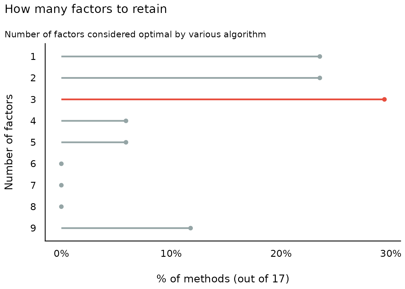
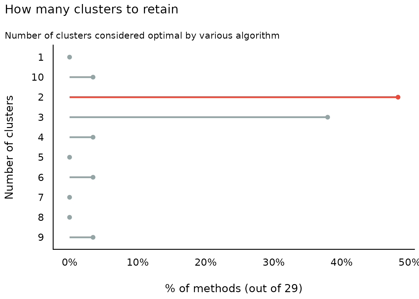
Number of Clusters to Retain
(related function documentation)
data(iris)
result <- n_clusters(standardize(iris[, 1:4]))
result
#> # Method Agreement Procedure:
#>
#> The choice of 2 clusters is supported by 13 (44.83%) methods out of 29 (Elbow, Gap_Maechler2012, Ch, DB, Duda, Pseudot2, Beale, Ratkowsky, PtBiserial, Mcclain, Dunn, SDindex, Mixture (VVV)).

plot(result)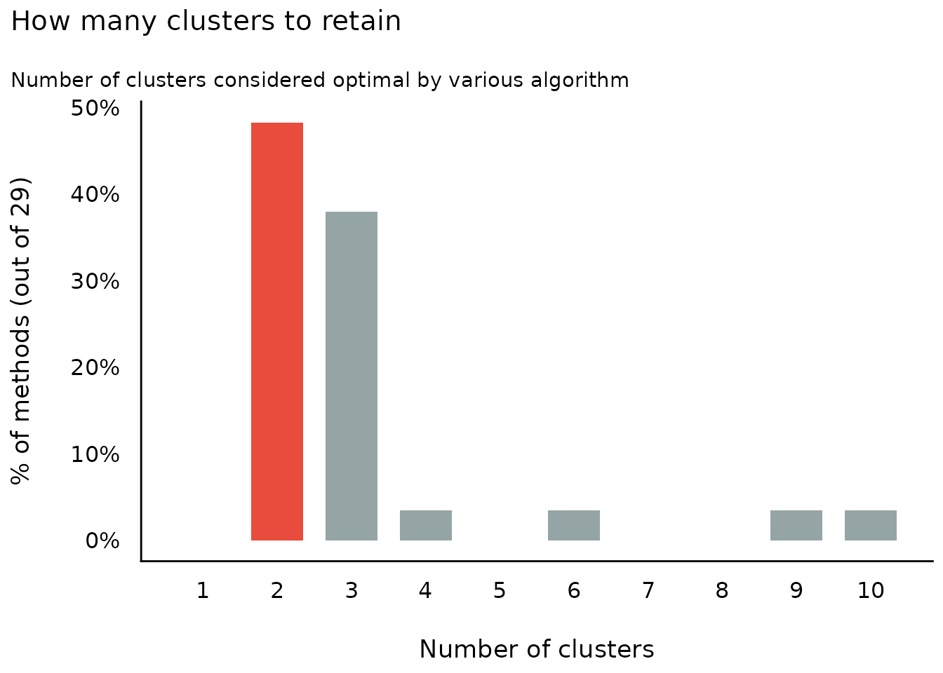
plot(result, type = "line")