Bayesian p-value based on the density at the Maximum A Posteriori (MAP)

Compute a Bayesian equivalent of the p-value, related to the odds that a parameter (described by its posterior distribution) has against the null hypothesis (h0) using Mills' (2014, 2017) Objective Bayesian Hypothesis Testing framework. It corresponds to the density value at the null (e.g., 0) divided by the density at the Maximum A Posteriori (MAP).

Usage

p_map(x, ...)

p_pointnull(x, ...)

# S3 method for class 'numeric'
p_map(x, null = 0, precision = 2^10, method = "kernel", ...)

# S3 method for class 'get_predicted'
p_map(
  x,
  null = 0,
  precision = 2^10,
  method = "kernel",
  use_iterations = FALSE,
  verbose = TRUE,
  ...
)

# S3 method for class 'data.frame'
p_map(x, null = 0, precision = 2^10, method = "kernel", rvar_col = NULL, ...)

# S3 method for class 'brmsfit'
p_map(
  x,
  null = 0,
  precision = 2^10,
  method = "kernel",
  effects = "fixed",
  component = "conditional",
  parameters = NULL,
  ...
)

Arguments

x

Vector representing a posterior distribution, or a data frame of such vectors. Can also be a Bayesian model. bayestestR supports a wide range of models (see, for example, methods("hdi")) and not all of those are documented in the 'Usage' section, because methods for other classes mostly resemble the arguments of the .numeric or .data.framemethods.

...

Currently not used.

null

The value considered as a "null" effect. Traditionally 0, but could also be 1 in the case of ratios of change (OR, IRR, ...).

precision

Number of points of density data. See the n parameter in density.

method

Density estimation method. Can be "kernel" (default), "logspline" or "KernSmooth".

use_iterations

Logical, if TRUE and x is a get_predicted object, (returned by insight::get_predicted()), the function is applied to the iterations instead of the predictions. This only applies to models that return iterations for predicted values (e.g., brmsfit models).

verbose

Toggle off warnings.

rvar_col

A single character - the name of an rvar column in the data frame to be processed. See example in p_direction().

effects

Should results for fixed effects ("fixed", the default), random effects ("random") or both ("all") be returned? Only applies to mixed models. May be abbreviated.

component

Which type of parameters to return, such as parameters for the conditional model, the zero-inflated part of the model, the dispersion term, etc. See details in section Model Components. May be abbreviated. Note that the conditional component also refers to the count or mean component - names may differ, depending on the modeling package. There are three convenient shortcuts (not applicable to all model classes):

component = "all" returns all possible parameters.
If component = "location", location parameters such as conditional, zero_inflated, smooth_terms, or instruments are returned (everything that are fixed or random effects - depending on the effects argument - but no auxiliary parameters).
For component = "distributional" (or "auxiliary"), components like sigma, dispersion, beta or precision (and other auxiliary parameters) are returned.

parameters

Regular expression pattern that describes the parameters that should be returned. Meta-parameters (like lp__ or prior_) are filtered by default, so only parameters that typically appear in the summary() are returned. Use parameters to select specific parameters for the output.

Details

Note that this method is sensitive to the density estimation method (see the section in the examples below).

Strengths and Limitations

Strengths: Straightforward computation. Objective property of the posterior distribution.

Limitations: Limited information favoring the null hypothesis. Relates on density approximation. Indirect relationship between mathematical definition and interpretation. Only suitable for weak / very diffused priors.

Model components

Possible values for the component argument depend on the model class. Following are valid options:

"all": returns all model components, applies to all models, but will only have an effect for models with more than just the conditional model component.
"conditional": only returns the conditional component, i.e. "fixed effects" terms from the model. Will only have an effect for models with more than just the conditional model component.
"smooth_terms": returns smooth terms, only applies to GAMs (or similar models that may contain smooth terms).
"zero_inflated" (or "zi"): returns the zero-inflation component.
"location": returns location parameters such as conditional, zero_inflated, or smooth_terms (everything that are fixed or random effects - depending on the effects argument - but no auxiliary parameters).
"distributional" (or "auxiliary"): components like sigma, dispersion, beta or precision (and other auxiliary parameters) are returned.

For models of class brmsfit (package brms), even more options are possible for the component argument, which are not all documented in detail here. See also ?insight::find_parameters.

References

Makowski D, Ben-Shachar MS, Chen SHA, Lüdecke D (2019) Indices of Effect Existence and Significance in the Bayesian Framework. Frontiers in Psychology 2019;10:2767. doi:10.3389/fpsyg.2019.02767
Mills, J. A. (2018). Objective Bayesian Precise Hypothesis Testing. University of Cincinnati.

Examples

library(bayestestR)

p_map(rnorm(1000, 0, 1))
#> MAP-based p-value
#> 
#> Parameter | p (MAP)
#> -------------------
#> Posterior |   0.998
p_map(rnorm(1000, 10, 1))
#> MAP-based p-value
#> 
#> Parameter | p (MAP)
#> -------------------
#> Posterior |  < .001
# \donttest{
model <- suppressWarnings(
  rstanarm::stan_glm(mpg ~ wt + gear, data = mtcars, chains = 2, iter = 200, refresh = 0)
)
p_map(model)
#> MAP-based p-value 
#> 
#> Parameter   | p (MAP)
#> ---------------------
#> (Intercept) |  < .001
#> wt          |  < .001
#> gear        |  0.963 

p_map(suppressWarnings(
  emmeans::emtrends(model, ~1, "wt", data = mtcars)
))
#> MAP-based p-value
#> 
#> X1      | p (MAP)
#> -----------------
#> overall |  < .001

model <- brms::brm(mpg ~ wt + cyl, data = mtcars)
#> Compiling Stan program...
#> Start sampling
#> 
#> SAMPLING FOR MODEL 'anon_model' NOW (CHAIN 1).
#> Chain 1: 
#> Chain 1: Gradient evaluation took 6e-06 seconds
#> Chain 1: 1000 transitions using 10 leapfrog steps per transition would take 0.06 seconds.
#> Chain 1: Adjust your expectations accordingly!
#> Chain 1: 
#> Chain 1: 
#> Chain 1: Iteration:    1 / 2000 [  0%]  (Warmup)
#> Chain 1: Iteration:  200 / 2000 [ 10%]  (Warmup)
#> Chain 1: Iteration:  400 / 2000 [ 20%]  (Warmup)
#> Chain 1: Iteration:  600 / 2000 [ 30%]  (Warmup)
#> Chain 1: Iteration:  800 / 2000 [ 40%]  (Warmup)
#> Chain 1: Iteration: 1000 / 2000 [ 50%]  (Warmup)
#> Chain 1: Iteration: 1001 / 2000 [ 50%]  (Sampling)
#> Chain 1: Iteration: 1200 / 2000 [ 60%]  (Sampling)
#> Chain 1: Iteration: 1400 / 2000 [ 70%]  (Sampling)
#> Chain 1: Iteration: 1600 / 2000 [ 80%]  (Sampling)
#> Chain 1: Iteration: 1800 / 2000 [ 90%]  (Sampling)
#> Chain 1: Iteration: 2000 / 2000 [100%]  (Sampling)
#> Chain 1: 
#> Chain 1:  Elapsed Time: 0.021 seconds (Warm-up)
#> Chain 1:                0.017 seconds (Sampling)
#> Chain 1:                0.038 seconds (Total)
#> Chain 1: 
#> 
#> SAMPLING FOR MODEL 'anon_model' NOW (CHAIN 2).
#> Chain 2: 
#> Chain 2: Gradient evaluation took 3e-06 seconds
#> Chain 2: 1000 transitions using 10 leapfrog steps per transition would take 0.03 seconds.
#> Chain 2: Adjust your expectations accordingly!
#> Chain 2: 
#> Chain 2: 
#> Chain 2: Iteration:    1 / 2000 [  0%]  (Warmup)
#> Chain 2: Iteration:  200 / 2000 [ 10%]  (Warmup)
#> Chain 2: Iteration:  400 / 2000 [ 20%]  (Warmup)
#> Chain 2: Iteration:  600 / 2000 [ 30%]  (Warmup)
#> Chain 2: Iteration:  800 / 2000 [ 40%]  (Warmup)
#> Chain 2: Iteration: 1000 / 2000 [ 50%]  (Warmup)
#> Chain 2: Iteration: 1001 / 2000 [ 50%]  (Sampling)
#> Chain 2: Iteration: 1200 / 2000 [ 60%]  (Sampling)
#> Chain 2: Iteration: 1400 / 2000 [ 70%]  (Sampling)
#> Chain 2: Iteration: 1600 / 2000 [ 80%]  (Sampling)
#> Chain 2: Iteration: 1800 / 2000 [ 90%]  (Sampling)
#> Chain 2: Iteration: 2000 / 2000 [100%]  (Sampling)
#> Chain 2: 
#> Chain 2:  Elapsed Time: 0.019 seconds (Warm-up)
#> Chain 2:                0.017 seconds (Sampling)
#> Chain 2:                0.036 seconds (Total)
#> Chain 2: 
#> 
#> SAMPLING FOR MODEL 'anon_model' NOW (CHAIN 3).
#> Chain 3: 
#> Chain 3: Gradient evaluation took 3e-06 seconds
#> Chain 3: 1000 transitions using 10 leapfrog steps per transition would take 0.03 seconds.
#> Chain 3: Adjust your expectations accordingly!
#> Chain 3: 
#> Chain 3: 
#> Chain 3: Iteration:    1 / 2000 [  0%]  (Warmup)
#> Chain 3: Iteration:  200 / 2000 [ 10%]  (Warmup)
#> Chain 3: Iteration:  400 / 2000 [ 20%]  (Warmup)
#> Chain 3: Iteration:  600 / 2000 [ 30%]  (Warmup)
#> Chain 3: Iteration:  800 / 2000 [ 40%]  (Warmup)
#> Chain 3: Iteration: 1000 / 2000 [ 50%]  (Warmup)
#> Chain 3: Iteration: 1001 / 2000 [ 50%]  (Sampling)
#> Chain 3: Iteration: 1200 / 2000 [ 60%]  (Sampling)
#> Chain 3: Iteration: 1400 / 2000 [ 70%]  (Sampling)
#> Chain 3: Iteration: 1600 / 2000 [ 80%]  (Sampling)
#> Chain 3: Iteration: 1800 / 2000 [ 90%]  (Sampling)
#> Chain 3: Iteration: 2000 / 2000 [100%]  (Sampling)
#> Chain 3: 
#> Chain 3:  Elapsed Time: 0.02 seconds (Warm-up)
#> Chain 3:                0.02 seconds (Sampling)
#> Chain 3:                0.04 seconds (Total)
#> Chain 3: 
#> 
#> SAMPLING FOR MODEL 'anon_model' NOW (CHAIN 4).
#> Chain 4: 
#> Chain 4: Gradient evaluation took 3e-06 seconds
#> Chain 4: 1000 transitions using 10 leapfrog steps per transition would take 0.03 seconds.
#> Chain 4: Adjust your expectations accordingly!
#> Chain 4: 
#> Chain 4: 
#> Chain 4: Iteration:    1 / 2000 [  0%]  (Warmup)
#> Chain 4: Iteration:  200 / 2000 [ 10%]  (Warmup)
#> Chain 4: Iteration:  400 / 2000 [ 20%]  (Warmup)
#> Chain 4: Iteration:  600 / 2000 [ 30%]  (Warmup)
#> Chain 4: Iteration:  800 / 2000 [ 40%]  (Warmup)
#> Chain 4: Iteration: 1000 / 2000 [ 50%]  (Warmup)
#> Chain 4: Iteration: 1001 / 2000 [ 50%]  (Sampling)
#> Chain 4: Iteration: 1200 / 2000 [ 60%]  (Sampling)
#> Chain 4: Iteration: 1400 / 2000 [ 70%]  (Sampling)
#> Chain 4: Iteration: 1600 / 2000 [ 80%]  (Sampling)
#> Chain 4: Iteration: 1800 / 2000 [ 90%]  (Sampling)
#> Chain 4: Iteration: 2000 / 2000 [100%]  (Sampling)
#> Chain 4: 
#> Chain 4:  Elapsed Time: 0.019 seconds (Warm-up)
#> Chain 4:                0.02 seconds (Sampling)
#> Chain 4:                0.039 seconds (Total)
#> Chain 4: 
p_map(model)
#> MAP-based p-value 
#> 
#> Parameter   | p (MAP)
#> ---------------------
#> (Intercept) |  < .001
#> wt          |  0.002 
#> cyl         |  0.005 

bf <- BayesFactor::ttestBF(x = rnorm(100, 1, 1))
p_map(bf)
#> MAP-based p-value
#> 
#> Parameter  | p (MAP)
#> --------------------
#> Difference |  < .001

# ---------------------------------------
# Robustness to density estimation method
set.seed(333)
data <- data.frame()
for (iteration in 1:250) {
  x <- rnorm(1000, 1, 1)
  result <- data.frame(
    Kernel = as.numeric(p_map(x, method = "kernel")),
    KernSmooth = as.numeric(p_map(x, method = "KernSmooth")),
    logspline = as.numeric(p_map(x, method = "logspline"))
  )
  data <- rbind(data, result)
}
data$KernSmooth <- data$Kernel - data$KernSmooth
data$logspline <- data$Kernel - data$logspline

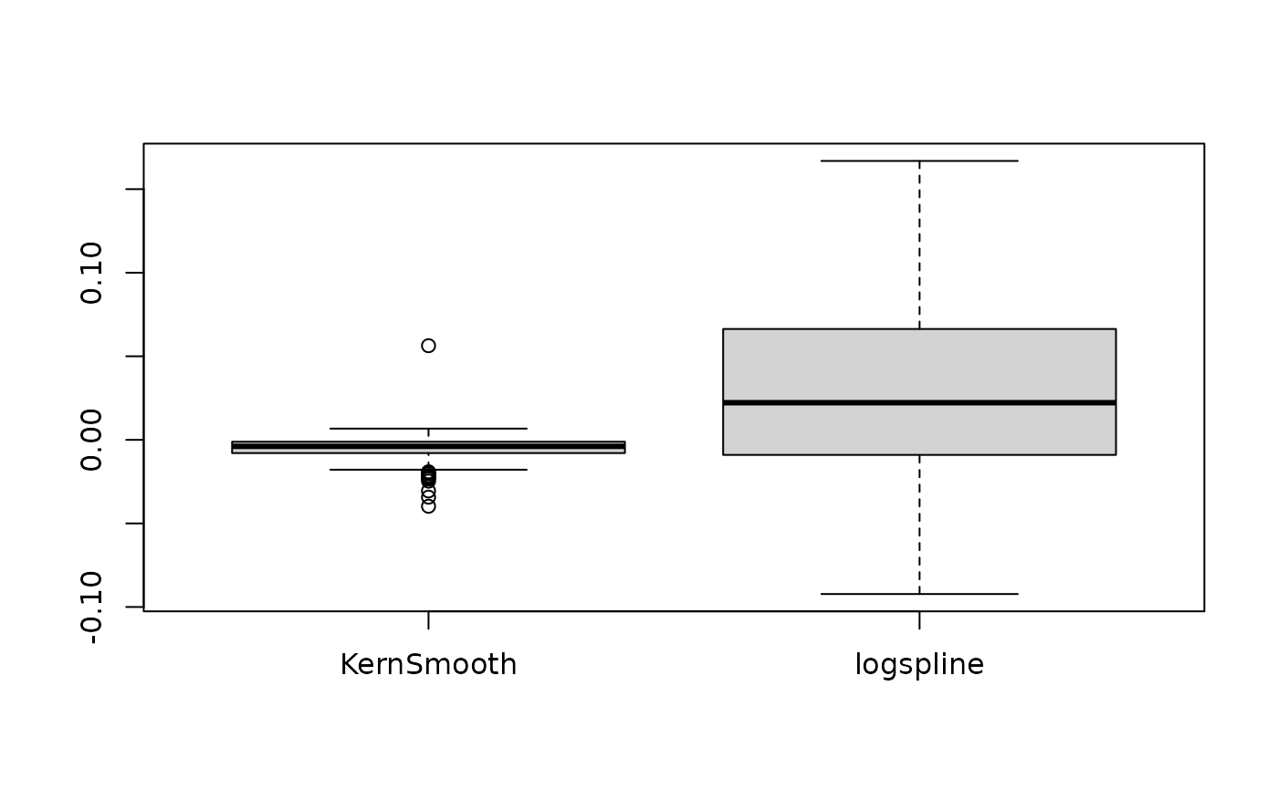
summary(data$KernSmooth)
#>      Min.   1st Qu.    Median      Mean   3rd Qu.      Max. 
#> -0.039724 -0.007909 -0.003885 -0.005338 -0.001128  0.056325 
summary(data$logspline)
#>      Min.   1st Qu.    Median      Mean   3rd Qu.      Max. 
#> -0.092243 -0.009008  0.022214  0.026966  0.066303  0.166870 
boxplot(data[c("KernSmooth", "logspline")])

# }