Bayes Factors (BF) for Order Restricted Models
Source:R/bayesfactor_restricted.R
bayesfactor_restricted.RdThis method computes Bayes factors for comparing a model with an order restrictions on its parameters
with the fully unrestricted model. Note that this method should only be used for confirmatory analyses.
The bf_* function is an alias of the main function.
For more info, see the Bayes factors vignette.
Usage
bayesfactor_restricted(posterior, ...)

bf_restricted(posterior, ...)

# S3 method for class 'stanreg'
bayesfactor_restricted(
  posterior,
  hypothesis,
  prior = NULL,
  verbose = TRUE,
  effects = "fixed",
  component = "conditional",
  ...
)

# S3 method for class 'brmsfit'
bayesfactor_restricted(
  posterior,
  hypothesis,
  prior = NULL,
  verbose = TRUE,
  effects = "fixed",
  component = "conditional",
  ...
)

# S3 method for class 'blavaan'
bayesfactor_restricted(
  posterior,
  hypothesis,
  prior = NULL,
  verbose = TRUE,
  ...
)

# S3 method for class 'emmGrid'
bayesfactor_restricted(
  posterior,
  hypothesis,
  prior = NULL,
  verbose = TRUE,
  ...
)

# S3 method for class 'matrix'
bayesfactor_restricted(
  posterior,
  hypothesis,
  prior = NULL,
  verbose = TRUE,
  ...
)

# S3 method for class 'data.frame'
bayesfactor_restricted(
  posterior,
  hypothesis,
  prior = NULL,
  rvar_col = NULL,
  ...
)
Arguments
- posterior
A
stanreg/brmsfitobject,emmGridor a data frame - representing a posterior distribution(s) from (see Details).- ...
Currently not used.
- hypothesis
A character vector specifying the restrictions as logical conditions (see examples below).
- prior
An object representing a prior distribution (see Details).
- verbose
Toggle off warnings.
- effects
Should variables for fixed effects (
"fixed"), random effects ("random") or both ("all") be returned? Only applies to mixed models. May be abbreviated.For models of from packages brms or rstanarm there are additional options:
"fixed"returns fixed effects."random_variance"return random effects parameters (variance and correlation components, e.g. those parameters that start withsd_orcor_)."grouplevel"returns random effects group level estimates, i.e. those parameters that start withr_."random"returns both"random_variance"and"grouplevel"."all"returns fixed effects and random effects variances."full"returns all parameters.
- component
Which type of parameters to return, such as parameters for the conditional model, the zero-inflated part of the model, the dispersion term, etc. See details in section Model Components. May be abbreviated. Note that the conditional component also refers to the count or mean component - names may differ, depending on the modeling package. There are three convenient shortcuts (not applicable to all model classes):
component = "all"returns all possible parameters.If
component = "location", location parameters such asconditional,zero_inflated,smooth_terms, orinstrumentsare returned (everything that are fixed or random effects - depending on theeffectsargument - but no auxiliary parameters).For
component = "distributional"(or"auxiliary"), components likesigma,dispersion,betaorprecision(and other auxiliary parameters) are returned.
- rvar_col
A single character - the name of an
rvarcolumn in the data frame to be processed. See example inp_direction().
Value
A data frame containing the (log) Bayes factor representing evidence
against the un-restricted model (Use as.numeric() to extract the
non-log Bayes factors; see examples). (A bool_results attribute contains
the results for each sample, indicating if they are included or not in the
hypothesized restriction.)
Details
This method is used to compute Bayes factors for order-restricted
models vs un-restricted models by setting an order restriction on the prior
and posterior distributions (Morey & Wagenmakers, 2013).
(Though it is possible to use bayesfactor_restricted() to test interval restrictions,
it is more suitable for testing order restrictions; see examples).
Additional methods
The resulting output is supported by the following methods:
as.matrix(): Extract a full matrix of (log-)Bayes factors between all models (using the transitivity of Bayes factors).as.logical(): Extract boolean vectors indicating which (prior/posterior) samples are included in the hypothesized restriction.as.numeric(): Extract the (possibly log-)Bayes factor values.
See examples and bayesfactor_methods.
Obtaining prior samples
It is important to provide the correct prior for meaningful results,
to match the posterior-type input:
A numeric vector -
priorshould also be a numeric vector, representing the prior-distributionA data frame -
priorshould also be a data frame, representing the prior-estimates, in matching column order.If
rvar_colis specified,priorshould be the name of anrvarcolumn that represents the prior-estimates.
Supported Bayesian model (
stanreg,brmsfit, etc.)priorshould be a model an equivalent model with MCMC samples from the priors only. Seeunupdate().If
prioris set toNULL,unupdate()is called internally (not supported forbrmsfit_multiplemodel).
Output from a
{marginaleffects}function -priorshould also be an equivalent output from a{marginaleffects}function based on a prior-model (Seeunupdate()).Output from an
{emmeans}functionpriorshould also be an equivalent output from an{emmeans}function based on a prior-model (Seeunupdate()).priorcan also be the original (posterior) model, in which case the function will try to "unupdate" the estimates (not supported if the estimates have undergone any transformations –"log","response", etc. – or anyregriding).
Transitivity of Bayes factors
For multiple inputs (models or hypotheses), the function will return multiple
Bayes factors between each model and the same reference model (the
denominator or un-restricted model). However, we can take advantage of the
transitivity of Bayes factors - where if we have two Bayes factors for Model
A and model B against the same reference model C, we can obtain a Bayes
factor for comparing model A to model B by dividing them:
$$BF_{AB} = \frac{BF_{AC}}{BF_{BC}} = \frac{\frac{ML_{A}}{ML_{C}}}{\frac{ML_{B}}{ML_{C}}} = \frac{ML_{A}}{ML_{B}}$$
(Where ML is the marginal likelihood.)
A full matrix comparing all models can be obtained with as.matrix().
Interpreting Bayes Factors
A Bayes factor greater than 1 can be interpreted as evidence against the
null, at which one convention is that a Bayes factor greater than 3 can be
considered as "substantial" evidence against the null (and vice versa, a
Bayes factor smaller than 1/3 indicates substantial evidence in favor of the
null-model). See also effectsize::interpret_bf().
References
Morey, R. D., & Wagenmakers, E. J. (2014). Simple relation between Bayesian order-restricted and point-null hypothesis tests. Statistics & Probability Letters, 92, 121-124.
Morey, R. D., & Rouder, J. N. (2011). Bayes factor approaches for testing interval null hypotheses. Psychological methods, 16(4), 406.
Morey, R. D. (Jan, 2015). Multiple Comparisons with BayesFactor, Part 2 – order restrictions. Retrieved from https://richarddmorey.org/category/order-restrictions/.
See also
Other Bayes factors:
bayesfactor_inclusion(),
bayesfactor_models(),
bayesfactor_parameters()
Examples
set.seed(444)
library(bayestestR)
prior <- data.frame(
A = rnorm(500),
B = rnorm(500),
C = rnorm(500)
)
posterior <- data.frame(
A = rnorm(500, .4, 0.7),
B = rnorm(500, -.2, 0.4),
C = rnorm(500, 0, 0.5)
)
hyps <- c(
"A > B & B > C",
"A > B & A > C",
"C > A"
)
(b <- bayesfactor_restricted(posterior, hypothesis = hyps, prior = prior))
#> Bayes Factor (Order-Restriction)
#>
#> Hypothesis P(Prior) P(Posterior) BF
#> A > B & B > C 0.16 0.23 1.39
#> A > B & A > C 0.36 0.59 1.61
#> C > A 0.46 0.34 0.742
#>
#> * Bayes factors for the restricted model vs. the un-restricted model.
# See the matrix of BFs
as.matrix(b)
#> # Bayes Factors for Restricted Models
#>
#> Denominator\Numerator | [1] | [2] | [3] | [4]
#> -----------------------------------------------------
#> [1] (Un-restricted) | 1 | 1.39 | 1.61 | 0.742
#> [2] A > B & B > C | 0.719 | 1 | 1.16 | 0.534
#> [3] A > B & A > C | 0.621 | 0.864 | 1 | 0.461
#> [4] C > A | 1.35 | 1.87 | 2.17 | 1
bool <- as.logical(b, which = "posterior")
head(bool)
#> A > B & B > C A > B & A > C C > A
#> [1,] TRUE TRUE FALSE
#> [2,] TRUE TRUE FALSE
#> [3,] TRUE TRUE FALSE
#> [4,] FALSE TRUE FALSE
#> [5,] FALSE FALSE TRUE
#> [6,] FALSE TRUE FALSE
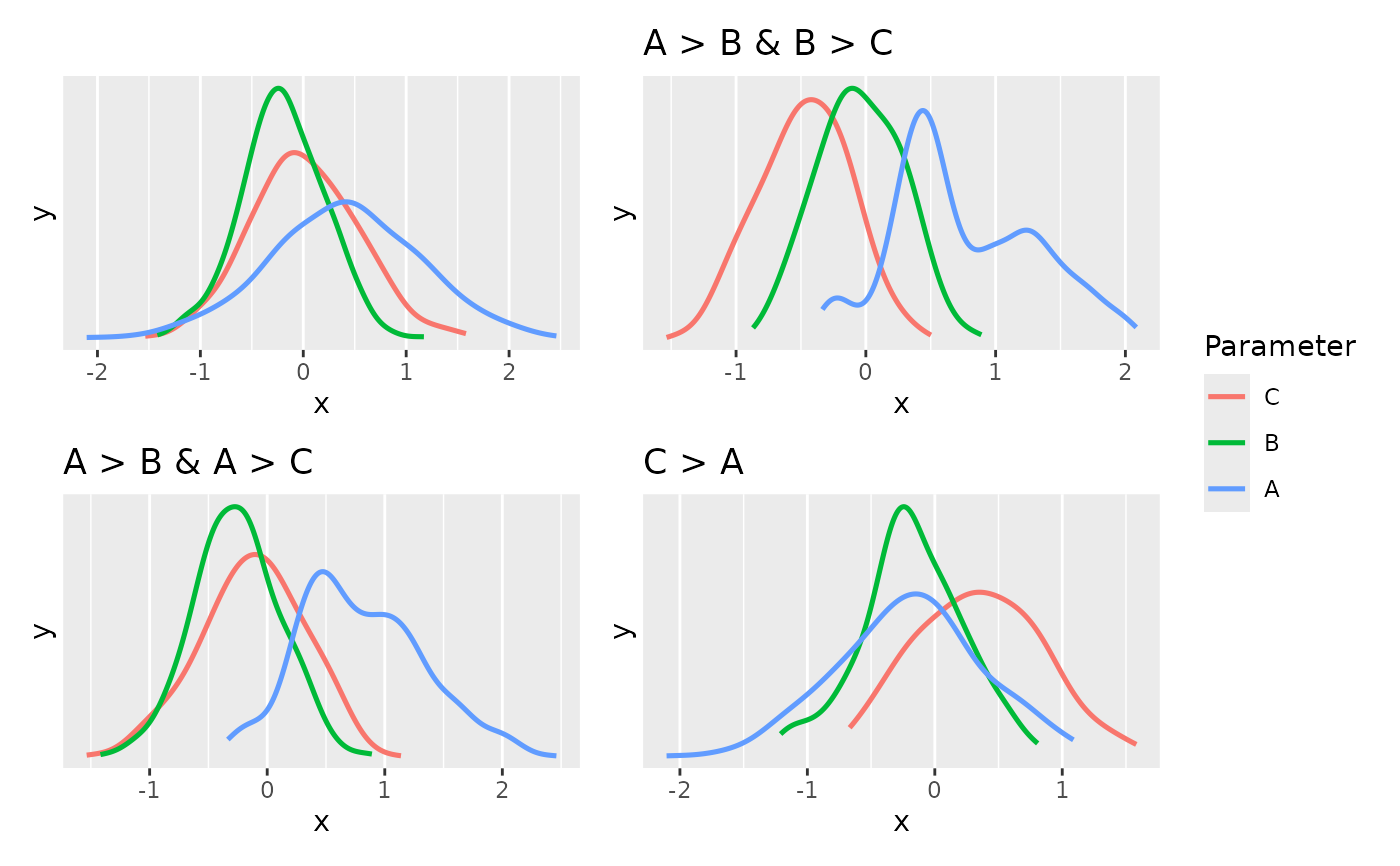
see::plots(
plot(estimate_density(posterior)),
# distribution **conditional** on the restrictions
plot(estimate_density(posterior[bool[, hyps[1]], ])) + ggplot2::ggtitle(hyps[1]),
plot(estimate_density(posterior[bool[, hyps[2]], ])) + ggplot2::ggtitle(hyps[2]),
plot(estimate_density(posterior[bool[, hyps[3]], ])) + ggplot2::ggtitle(hyps[3]),
guides = "collect"
)
 # \donttest{
# rstanarm models
# ---------------
data("mtcars")
fit_stan <- rstanarm::stan_glm(mpg ~ wt + cyl + am,
data = mtcars, refresh = 0
)
hyps <- c(
"am > 0 & cyl < 0",
"cyl < 0",
"wt - cyl > 0"
)
bayesfactor_restricted(fit_stan, hypothesis = hyps)
#> Sampling priors, please wait...
#> Bayes Factor (Order-Restriction)
#>
#> Hypothesis P(Prior) P(Posterior) BF
#> am > 0 & cyl < 0 0.25 0.56 2.25
#> cyl < 0 0.50 1.00 1.99
#> wt - cyl > 0 0.50 0.10 0.197
#>
#> * Bayes factors for the restricted model vs. the un-restricted model.
# }
# \donttest{
# emmGrid objects
# ---------------
# replicating http://bayesfactor.blogspot.com/2015/01/multiple-comparisons-with-bayesfactor-2.html
data("disgust")
contrasts(disgust$condition) <- contr.equalprior_pairs # see vignette
fit_model <- rstanarm::stan_glm(score ~ condition, data = disgust, family = gaussian())
#>
#> SAMPLING FOR MODEL 'continuous' NOW (CHAIN 1).
#> Chain 1:
#> Chain 1: Gradient evaluation took 2.3e-05 seconds
#> Chain 1: 1000 transitions using 10 leapfrog steps per transition would take 0.23 seconds.
#> Chain 1: Adjust your expectations accordingly!
#> Chain 1:
#> Chain 1:
#> Chain 1: Iteration: 1 / 2000 [ 0%] (Warmup)
#> Chain 1: Iteration: 200 / 2000 [ 10%] (Warmup)
#> Chain 1: Iteration: 400 / 2000 [ 20%] (Warmup)
#> Chain 1: Iteration: 600 / 2000 [ 30%] (Warmup)
#> Chain 1: Iteration: 800 / 2000 [ 40%] (Warmup)
#> Chain 1: Iteration: 1000 / 2000 [ 50%] (Warmup)
#> Chain 1: Iteration: 1001 / 2000 [ 50%] (Sampling)
#> Chain 1: Iteration: 1200 / 2000 [ 60%] (Sampling)
#> Chain 1: Iteration: 1400 / 2000 [ 70%] (Sampling)
#> Chain 1: Iteration: 1600 / 2000 [ 80%] (Sampling)
#> Chain 1: Iteration: 1800 / 2000 [ 90%] (Sampling)
#> Chain 1: Iteration: 2000 / 2000 [100%] (Sampling)
#> Chain 1:
#> Chain 1: Elapsed Time: 0.03 seconds (Warm-up)
#> Chain 1: 0.039 seconds (Sampling)
#> Chain 1: 0.069 seconds (Total)
#> Chain 1:
#>
#> SAMPLING FOR MODEL 'continuous' NOW (CHAIN 2).
#> Chain 2:
#> Chain 2: Gradient evaluation took 1.4e-05 seconds
#> Chain 2: 1000 transitions using 10 leapfrog steps per transition would take 0.14 seconds.
#> Chain 2: Adjust your expectations accordingly!
#> Chain 2:
#> Chain 2:
#> Chain 2: Iteration: 1 / 2000 [ 0%] (Warmup)
#> Chain 2: Iteration: 200 / 2000 [ 10%] (Warmup)
#> Chain 2: Iteration: 400 / 2000 [ 20%] (Warmup)
#> Chain 2: Iteration: 600 / 2000 [ 30%] (Warmup)
#> Chain 2: Iteration: 800 / 2000 [ 40%] (Warmup)
#> Chain 2: Iteration: 1000 / 2000 [ 50%] (Warmup)
#> Chain 2: Iteration: 1001 / 2000 [ 50%] (Sampling)
#> Chain 2: Iteration: 1200 / 2000 [ 60%] (Sampling)
#> Chain 2: Iteration: 1400 / 2000 [ 70%] (Sampling)
#> Chain 2: Iteration: 1600 / 2000 [ 80%] (Sampling)
#> Chain 2: Iteration: 1800 / 2000 [ 90%] (Sampling)
#> Chain 2: Iteration: 2000 / 2000 [100%] (Sampling)
#> Chain 2:
#> Chain 2: Elapsed Time: 0.03 seconds (Warm-up)
#> Chain 2: 0.04 seconds (Sampling)
#> Chain 2: 0.07 seconds (Total)
#> Chain 2:
#>
#> SAMPLING FOR MODEL 'continuous' NOW (CHAIN 3).
#> Chain 3:
#> Chain 3: Gradient evaluation took 1.5e-05 seconds
#> Chain 3: 1000 transitions using 10 leapfrog steps per transition would take 0.15 seconds.
#> Chain 3: Adjust your expectations accordingly!
#> Chain 3:
#> Chain 3:
#> Chain 3: Iteration: 1 / 2000 [ 0%] (Warmup)
#> Chain 3: Iteration: 200 / 2000 [ 10%] (Warmup)
#> Chain 3: Iteration: 400 / 2000 [ 20%] (Warmup)
#> Chain 3: Iteration: 600 / 2000 [ 30%] (Warmup)
#> Chain 3: Iteration: 800 / 2000 [ 40%] (Warmup)
#> Chain 3: Iteration: 1000 / 2000 [ 50%] (Warmup)
#> Chain 3: Iteration: 1001 / 2000 [ 50%] (Sampling)
#> Chain 3: Iteration: 1200 / 2000 [ 60%] (Sampling)
#> Chain 3: Iteration: 1400 / 2000 [ 70%] (Sampling)
#> Chain 3: Iteration: 1600 / 2000 [ 80%] (Sampling)
#> Chain 3: Iteration: 1800 / 2000 [ 90%] (Sampling)
#> Chain 3: Iteration: 2000 / 2000 [100%] (Sampling)
#> Chain 3:
#> Chain 3: Elapsed Time: 0.03 seconds (Warm-up)
#> Chain 3: 0.039 seconds (Sampling)
#> Chain 3: 0.069 seconds (Total)
#> Chain 3:
#>
#> SAMPLING FOR MODEL 'continuous' NOW (CHAIN 4).
#> Chain 4:
#> Chain 4: Gradient evaluation took 1.1e-05 seconds
#> Chain 4: 1000 transitions using 10 leapfrog steps per transition would take 0.11 seconds.
#> Chain 4: Adjust your expectations accordingly!
#> Chain 4:
#> Chain 4:
#> Chain 4: Iteration: 1 / 2000 [ 0%] (Warmup)
#> Chain 4: Iteration: 200 / 2000 [ 10%] (Warmup)
#> Chain 4: Iteration: 400 / 2000 [ 20%] (Warmup)
#> Chain 4: Iteration: 600 / 2000 [ 30%] (Warmup)
#> Chain 4: Iteration: 800 / 2000 [ 40%] (Warmup)
#> Chain 4: Iteration: 1000 / 2000 [ 50%] (Warmup)
#> Chain 4: Iteration: 1001 / 2000 [ 50%] (Sampling)
#> Chain 4: Iteration: 1200 / 2000 [ 60%] (Sampling)
#> Chain 4: Iteration: 1400 / 2000 [ 70%] (Sampling)
#> Chain 4: Iteration: 1600 / 2000 [ 80%] (Sampling)
#> Chain 4: Iteration: 1800 / 2000 [ 90%] (Sampling)
#> Chain 4: Iteration: 2000 / 2000 [100%] (Sampling)
#> Chain 4:
#> Chain 4: Elapsed Time: 0.028 seconds (Warm-up)
#> Chain 4: 0.039 seconds (Sampling)
#> Chain 4: 0.067 seconds (Total)
#> Chain 4:
em_condition <- emmeans::emmeans(fit_model, ~condition, data = disgust)
hyps <- c("lemon < control & control < sulfur")
bayesfactor_restricted(em_condition, prior = fit_model, hypothesis = hyps)
#> Sampling priors, please wait...
#> Bayes Factor (Order-Restriction)
#>
#> Hypothesis P(Prior) P(Posterior) BF
#> lemon < control & control < sulfur 0.17 0.75 4.28
#>
#> * Bayes factors for the restricted model vs. the un-restricted model.
# > # Bayes Factor (Order-Restriction)
# >
# > Hypothesis P(Prior) P(Posterior) BF
# > lemon < control & control < sulfur 0.17 0.75 4.49
# > ---
# > Bayes factors for the restricted model vs. the un-restricted model.
# }
# \donttest{
# rstanarm models
# ---------------
data("mtcars")
fit_stan <- rstanarm::stan_glm(mpg ~ wt + cyl + am,
data = mtcars, refresh = 0
)
hyps <- c(
"am > 0 & cyl < 0",
"cyl < 0",
"wt - cyl > 0"
)
bayesfactor_restricted(fit_stan, hypothesis = hyps)
#> Sampling priors, please wait...
#> Bayes Factor (Order-Restriction)
#>
#> Hypothesis P(Prior) P(Posterior) BF
#> am > 0 & cyl < 0 0.25 0.56 2.25
#> cyl < 0 0.50 1.00 1.99
#> wt - cyl > 0 0.50 0.10 0.197
#>
#> * Bayes factors for the restricted model vs. the un-restricted model.
# }
# \donttest{
# emmGrid objects
# ---------------
# replicating http://bayesfactor.blogspot.com/2015/01/multiple-comparisons-with-bayesfactor-2.html
data("disgust")
contrasts(disgust$condition) <- contr.equalprior_pairs # see vignette
fit_model <- rstanarm::stan_glm(score ~ condition, data = disgust, family = gaussian())
#>
#> SAMPLING FOR MODEL 'continuous' NOW (CHAIN 1).
#> Chain 1:
#> Chain 1: Gradient evaluation took 2.3e-05 seconds
#> Chain 1: 1000 transitions using 10 leapfrog steps per transition would take 0.23 seconds.
#> Chain 1: Adjust your expectations accordingly!
#> Chain 1:
#> Chain 1:
#> Chain 1: Iteration: 1 / 2000 [ 0%] (Warmup)
#> Chain 1: Iteration: 200 / 2000 [ 10%] (Warmup)
#> Chain 1: Iteration: 400 / 2000 [ 20%] (Warmup)
#> Chain 1: Iteration: 600 / 2000 [ 30%] (Warmup)
#> Chain 1: Iteration: 800 / 2000 [ 40%] (Warmup)
#> Chain 1: Iteration: 1000 / 2000 [ 50%] (Warmup)
#> Chain 1: Iteration: 1001 / 2000 [ 50%] (Sampling)
#> Chain 1: Iteration: 1200 / 2000 [ 60%] (Sampling)
#> Chain 1: Iteration: 1400 / 2000 [ 70%] (Sampling)
#> Chain 1: Iteration: 1600 / 2000 [ 80%] (Sampling)
#> Chain 1: Iteration: 1800 / 2000 [ 90%] (Sampling)
#> Chain 1: Iteration: 2000 / 2000 [100%] (Sampling)
#> Chain 1:
#> Chain 1: Elapsed Time: 0.03 seconds (Warm-up)
#> Chain 1: 0.039 seconds (Sampling)
#> Chain 1: 0.069 seconds (Total)
#> Chain 1:
#>
#> SAMPLING FOR MODEL 'continuous' NOW (CHAIN 2).
#> Chain 2:
#> Chain 2: Gradient evaluation took 1.4e-05 seconds
#> Chain 2: 1000 transitions using 10 leapfrog steps per transition would take 0.14 seconds.
#> Chain 2: Adjust your expectations accordingly!
#> Chain 2:
#> Chain 2:
#> Chain 2: Iteration: 1 / 2000 [ 0%] (Warmup)
#> Chain 2: Iteration: 200 / 2000 [ 10%] (Warmup)
#> Chain 2: Iteration: 400 / 2000 [ 20%] (Warmup)
#> Chain 2: Iteration: 600 / 2000 [ 30%] (Warmup)
#> Chain 2: Iteration: 800 / 2000 [ 40%] (Warmup)
#> Chain 2: Iteration: 1000 / 2000 [ 50%] (Warmup)
#> Chain 2: Iteration: 1001 / 2000 [ 50%] (Sampling)
#> Chain 2: Iteration: 1200 / 2000 [ 60%] (Sampling)
#> Chain 2: Iteration: 1400 / 2000 [ 70%] (Sampling)
#> Chain 2: Iteration: 1600 / 2000 [ 80%] (Sampling)
#> Chain 2: Iteration: 1800 / 2000 [ 90%] (Sampling)
#> Chain 2: Iteration: 2000 / 2000 [100%] (Sampling)
#> Chain 2:
#> Chain 2: Elapsed Time: 0.03 seconds (Warm-up)
#> Chain 2: 0.04 seconds (Sampling)
#> Chain 2: 0.07 seconds (Total)
#> Chain 2:
#>
#> SAMPLING FOR MODEL 'continuous' NOW (CHAIN 3).
#> Chain 3:
#> Chain 3: Gradient evaluation took 1.5e-05 seconds
#> Chain 3: 1000 transitions using 10 leapfrog steps per transition would take 0.15 seconds.
#> Chain 3: Adjust your expectations accordingly!
#> Chain 3:
#> Chain 3:
#> Chain 3: Iteration: 1 / 2000 [ 0%] (Warmup)
#> Chain 3: Iteration: 200 / 2000 [ 10%] (Warmup)
#> Chain 3: Iteration: 400 / 2000 [ 20%] (Warmup)
#> Chain 3: Iteration: 600 / 2000 [ 30%] (Warmup)
#> Chain 3: Iteration: 800 / 2000 [ 40%] (Warmup)
#> Chain 3: Iteration: 1000 / 2000 [ 50%] (Warmup)
#> Chain 3: Iteration: 1001 / 2000 [ 50%] (Sampling)
#> Chain 3: Iteration: 1200 / 2000 [ 60%] (Sampling)
#> Chain 3: Iteration: 1400 / 2000 [ 70%] (Sampling)
#> Chain 3: Iteration: 1600 / 2000 [ 80%] (Sampling)
#> Chain 3: Iteration: 1800 / 2000 [ 90%] (Sampling)
#> Chain 3: Iteration: 2000 / 2000 [100%] (Sampling)
#> Chain 3:
#> Chain 3: Elapsed Time: 0.03 seconds (Warm-up)
#> Chain 3: 0.039 seconds (Sampling)
#> Chain 3: 0.069 seconds (Total)
#> Chain 3:
#>
#> SAMPLING FOR MODEL 'continuous' NOW (CHAIN 4).
#> Chain 4:
#> Chain 4: Gradient evaluation took 1.1e-05 seconds
#> Chain 4: 1000 transitions using 10 leapfrog steps per transition would take 0.11 seconds.
#> Chain 4: Adjust your expectations accordingly!
#> Chain 4:
#> Chain 4:
#> Chain 4: Iteration: 1 / 2000 [ 0%] (Warmup)
#> Chain 4: Iteration: 200 / 2000 [ 10%] (Warmup)
#> Chain 4: Iteration: 400 / 2000 [ 20%] (Warmup)
#> Chain 4: Iteration: 600 / 2000 [ 30%] (Warmup)
#> Chain 4: Iteration: 800 / 2000 [ 40%] (Warmup)
#> Chain 4: Iteration: 1000 / 2000 [ 50%] (Warmup)
#> Chain 4: Iteration: 1001 / 2000 [ 50%] (Sampling)
#> Chain 4: Iteration: 1200 / 2000 [ 60%] (Sampling)
#> Chain 4: Iteration: 1400 / 2000 [ 70%] (Sampling)
#> Chain 4: Iteration: 1600 / 2000 [ 80%] (Sampling)
#> Chain 4: Iteration: 1800 / 2000 [ 90%] (Sampling)
#> Chain 4: Iteration: 2000 / 2000 [100%] (Sampling)
#> Chain 4:
#> Chain 4: Elapsed Time: 0.028 seconds (Warm-up)
#> Chain 4: 0.039 seconds (Sampling)
#> Chain 4: 0.067 seconds (Total)
#> Chain 4:
em_condition <- emmeans::emmeans(fit_model, ~condition, data = disgust)
hyps <- c("lemon < control & control < sulfur")
bayesfactor_restricted(em_condition, prior = fit_model, hypothesis = hyps)
#> Sampling priors, please wait...
#> Bayes Factor (Order-Restriction)
#>
#> Hypothesis P(Prior) P(Posterior) BF
#> lemon < control & control < sulfur 0.17 0.75 4.28
#>
#> * Bayes factors for the restricted model vs. the un-restricted model.
# > # Bayes Factor (Order-Restriction)
# >
# > Hypothesis P(Prior) P(Posterior) BF
# > lemon < control & control < sulfur 0.17 0.75 4.49
# > ---
# > Bayes factors for the restricted model vs. the un-restricted model.
# }