This vignette can be referred to by citing the package:
citation("see")
#> To cite package 'see' in publications use:
#>
#>   Lüdecke et al., (2021). see: An R Package for Visualizing Statistical
#>   Models. Journal of Open Source Software, 6(64), 3393.
#>   https://doi.org/10.21105/joss.03393
#>
#> A BibTeX entry for LaTeX users is
#>
#>   @Article{,
#>     title = {{see}: An {R} Package for Visualizing Statistical Models},
#>     author = {Daniel Lüdecke and Indrajeet Patil and Mattan S. Ben-Shachar and Brenton M. Wiernik and Philip Waggoner and Dominique Makowski},
#>     journal = {Journal of Open Source Software},
#>     year = {2021},
#>     volume = {6},
#>     number = {64},
#>     pages = {3393},
#>     doi = {10.21105/joss.03393},
#>   }
Before we start, we create some data sets with three, four and five groups; one is useful to demonstrate line-geoms, the iris-dataset is used for point-geoms.
library(ggplot2)
library(see)

data(iris)
iris$group4 <- as.factor(sample(1:4, size = nrow(iris), replace = TRUE))
iris$group5 <- as.factor(sample(1:5, size = nrow(iris), replace = TRUE))

d1 <- data.frame(
  x = rep(1:20, 3),
  y = c(
    seq(2, 4, length.out = 20),
    seq(3, 6, length.out = 20),
    seq(5, 3, length.out = 20)
  ),
  group = rep(factor(1:3), each = 20)
)

d2 <- data.frame(
  x = rep(1:20, 4),
  y = c(
    seq(2, 4, length.out = 20),
    seq(3, 6, length.out = 20),
    seq(5, 3, length.out = 20),
    seq(4, 2.5, length.out = 20)
  ),
  group = rep(factor(1:4), each = 20)
)

d3 <- data.frame(
  x = rep(1:20, 5),
  y = c(
    seq(2, 4, length.out = 20),
    seq(3, 6, length.out = 20),
    seq(5, 3, length.out = 20),
    seq(4, 2.5, length.out = 20),
    seq(3.5, 4.5, length.out = 20)
  ),
  group = rep(factor(1:5), each = 20)
)

theme_set(theme_abyss(legend.position = "bottom"))
The see Color Scales
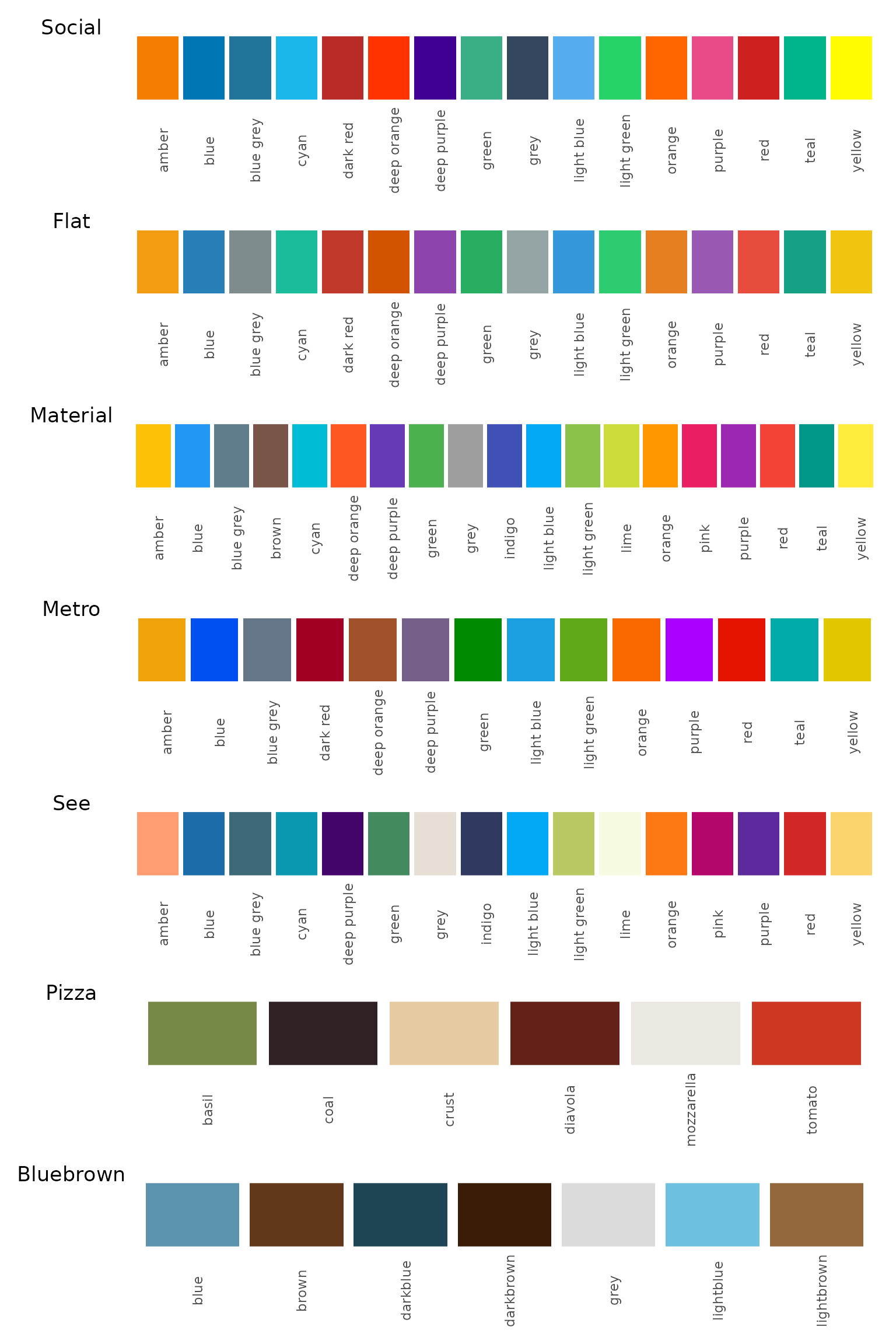
There are several different color
scales available in the see package, most of them having
some pre-defined palettes like "full", "ice",
"rainbow", "complement",
"contrast", or "light" - exceptions are the pizza
color scale and bluebrown
color scale.
In this vignettes, we show the "light" palettes for the
different color scales to give an impression how these scales work with
different type of data, especially for dark themes.
Social Colors - Three Groups
p1 <- ggplot(d1, aes(x, y, colour = group)) +
  geom_line(linewidth = 1) +
  scale_color_social(palette = "light")

p2 <- ggplot(iris, aes(Sepal.Length, Sepal.Width, colour = Species)) +
  geom_point2(size = 2.5) +
  scale_color_social(palette = "light")

plots(p1, p2, n_rows = 1)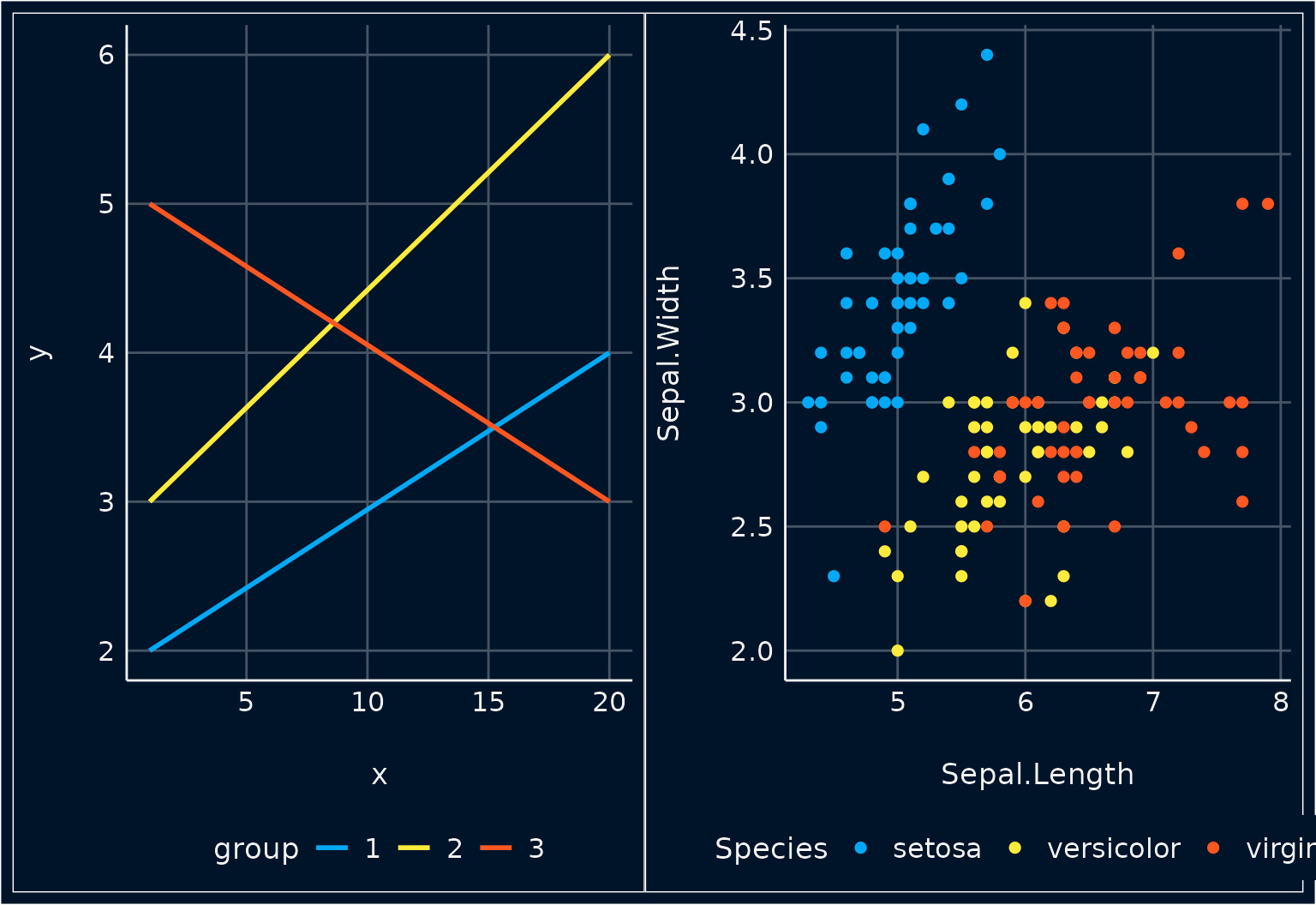
Social Colors - Four Groups
p1 <- ggplot(d2, aes(x, y, colour = group)) +
  geom_line(linewidth = 1) +
  scale_color_social(palette = "light")

p2 <- ggplot(iris, aes(Sepal.Length, Sepal.Width, colour = group4)) +
  geom_point2(size = 2.5) +
  scale_color_social(palette = "light")

plots(p1, p2, n_rows = 1)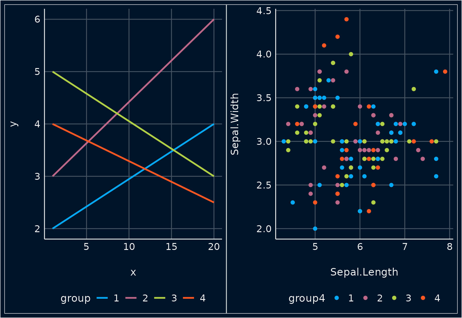
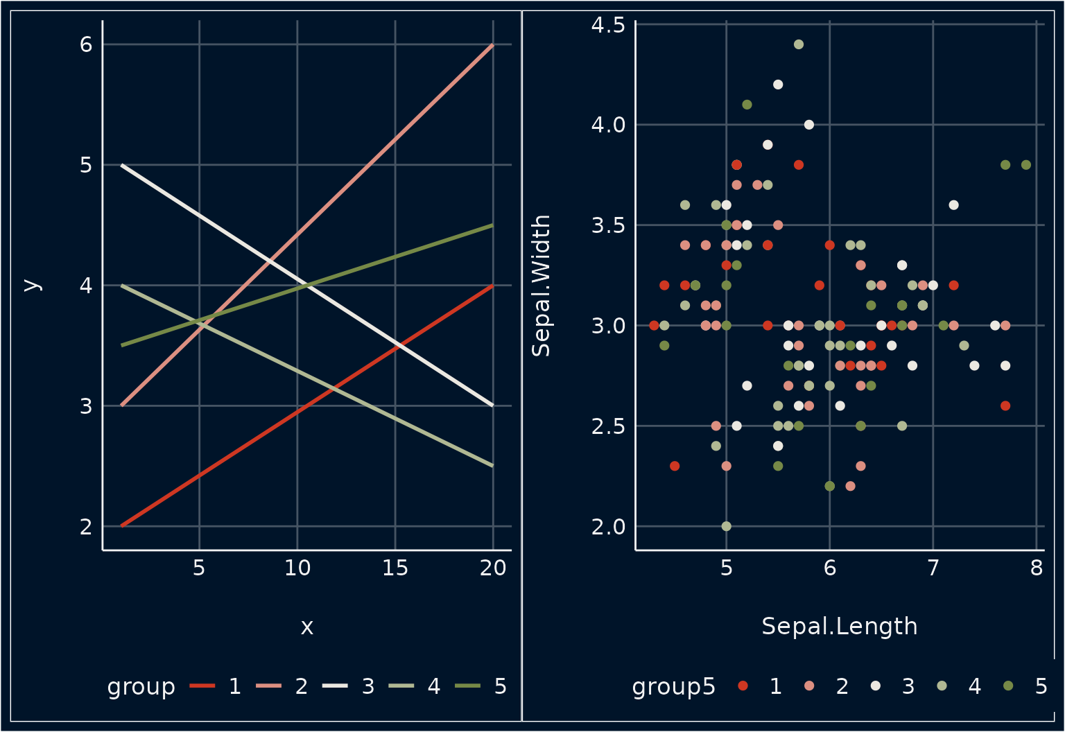
Social Colors - Five Groups
p1 <- ggplot(d3, aes(x, y, colour = group)) +
  geom_line(linewidth = 1) +
  scale_color_social(palette = "light")

p2 <- ggplot(iris, aes(Sepal.Length, Sepal.Width, colour = group5)) +
  geom_point2(size = 2.5) +
  scale_color_social(palette = "light")

plots(p1, p2, n_rows = 1)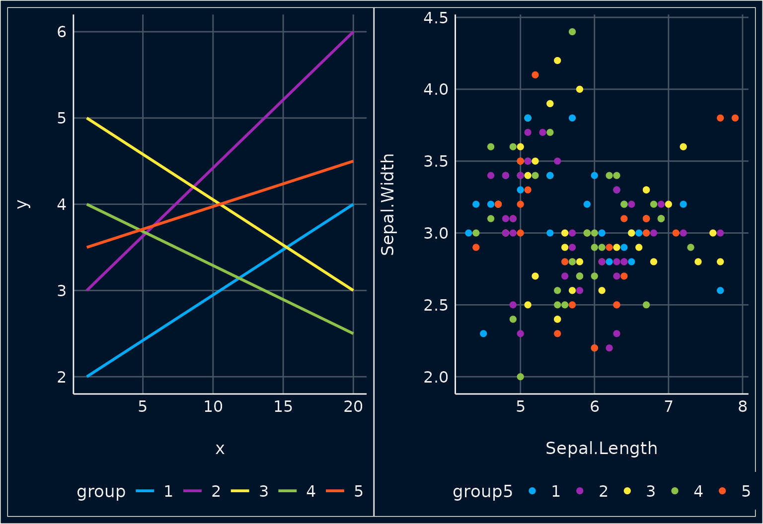
Material Colors
Material Colors - Three Groups
p1 <- ggplot(d1, aes(x, y, colour = group)) +
  geom_line(linewidth = 1) +
  scale_color_material(palette = "light")

p2 <- ggplot(iris, aes(Sepal.Length, Sepal.Width, colour = Species)) +
  geom_point2(size = 2.5) +
  scale_color_material(palette = "light")

plots(p1, p2, n_rows = 1)
Material Colors - Four Groups
p1 <- ggplot(d2, aes(x, y, colour = group)) +
  geom_line(linewidth = 1) +
  scale_color_material(palette = "light")

p2 <- ggplot(iris, aes(Sepal.Length, Sepal.Width, colour = group4)) +
  geom_point2(size = 2.5) +
  scale_color_material(palette = "light")

plots(p1, p2, n_rows = 1)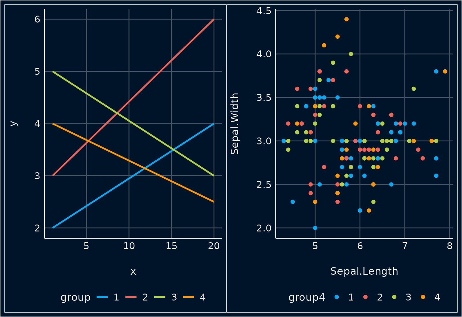
Material Colors - Five Groups
p1 <- ggplot(d3, aes(x, y, colour = group)) +
  geom_line(linewidth = 1) +
  scale_color_material(palette = "light")

p2 <- ggplot(iris, aes(Sepal.Length, Sepal.Width, colour = group5)) +
  geom_point2(size = 2.5) +
  scale_color_material(palette = "light")

plots(p1, p2, n_rows = 1)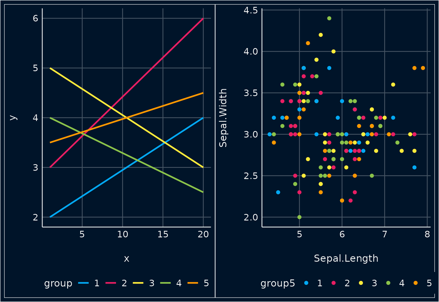
Flat Colors
Flat Colors - Three Groups
p1 <- ggplot(d1, aes(x, y, colour = group)) +
  geom_line(linewidth = 1) +
  scale_color_flat(palette = "light")

p2 <- ggplot(iris, aes(Sepal.Length, Sepal.Width, colour = Species)) +
  geom_point2(size = 2.5) +
  scale_color_flat(palette = "light")

plots(p1, p2, n_rows = 1)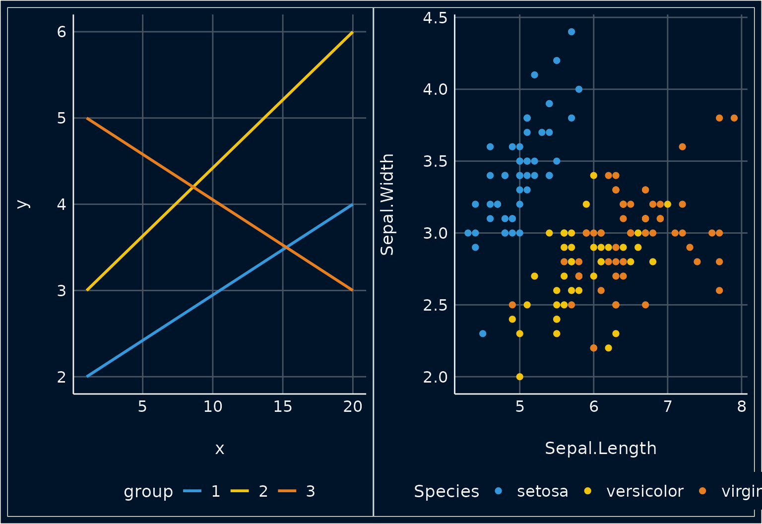
Flat Colors - Four Groups
p1 <- ggplot(d2, aes(x, y, colour = group)) +
  geom_line(linewidth = 1) +
  scale_color_flat(palette = "light")

p2 <- ggplot(iris, aes(Sepal.Length, Sepal.Width, colour = group4)) +
  geom_point2(size = 2.5) +
  scale_color_flat(palette = "light")

plots(p1, p2, n_rows = 1)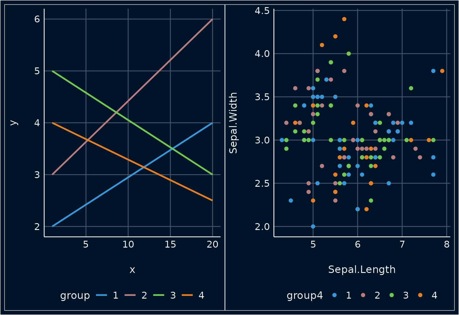
Flat Colors - Five Groups
p1 <- ggplot(d3, aes(x, y, colour = group)) +
  geom_line(linewidth = 1) +
  scale_color_flat(palette = "light")

p2 <- ggplot(iris, aes(Sepal.Length, Sepal.Width, colour = group5)) +
  geom_point2(size = 2.5) +
  scale_color_flat(palette = "light")

plots(p1, p2, n_rows = 1)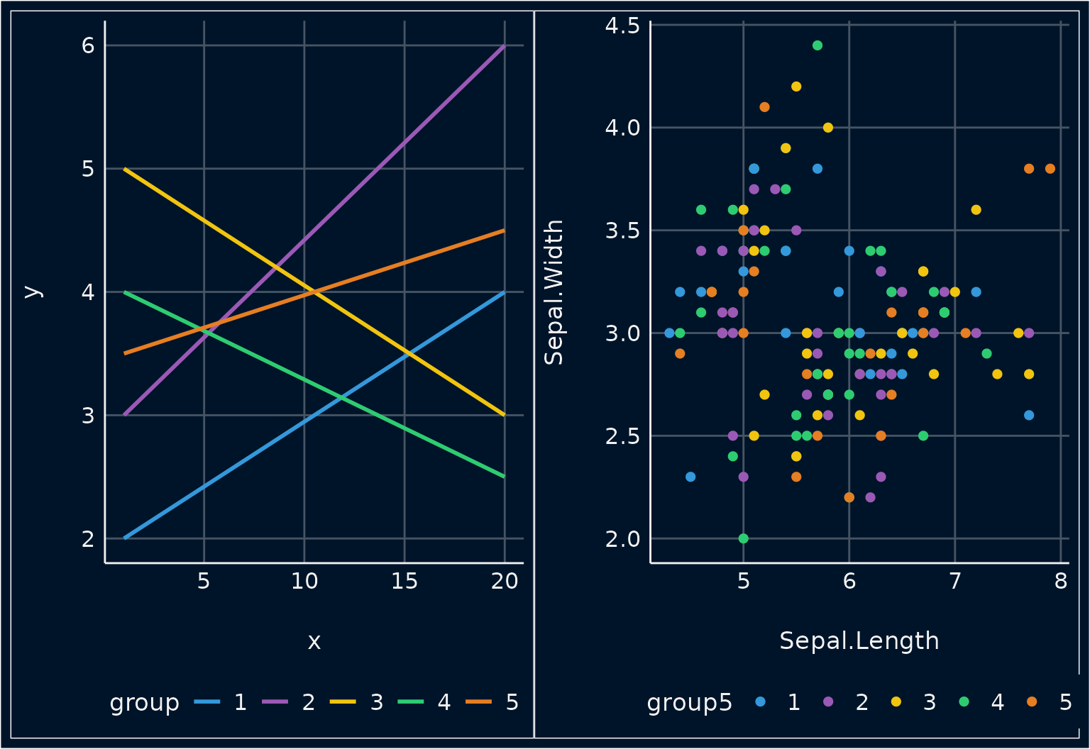
Metro Colors
Metro Colors - Three Groups
p1 <- ggplot(d1, aes(x, y, colour = group)) +
  geom_line(linewidth = 1) +
  scale_color_metro(palette = "light")

p2 <- ggplot(iris, aes(Sepal.Length, Sepal.Width, colour = Species)) +
  geom_point2(size = 2.5) +
  scale_color_metro(palette = "light")

plots(p1, p2, n_rows = 1)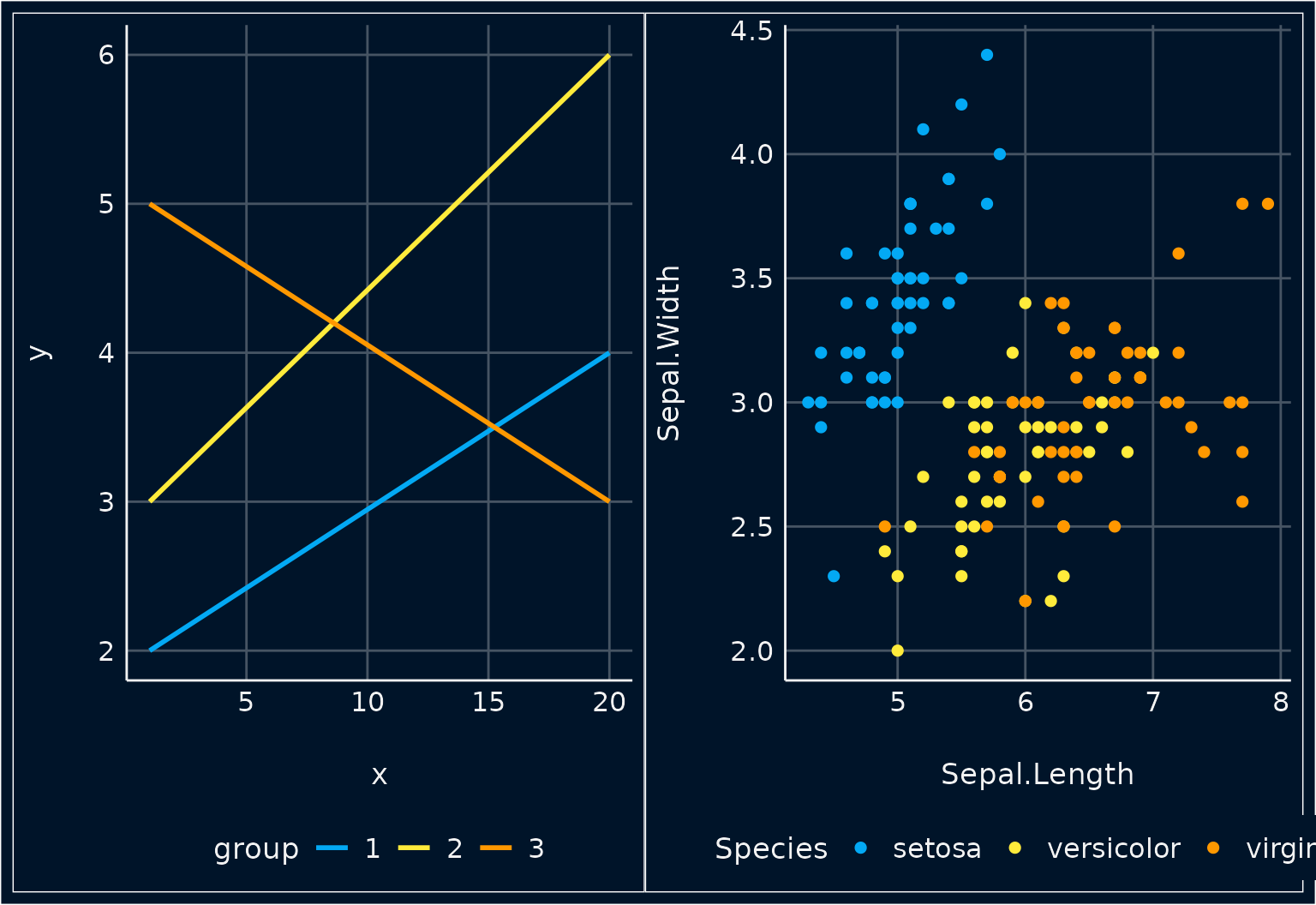
Metro Colors - Four Groups
p1 <- ggplot(d2, aes(x, y, colour = group)) +
  geom_line(linewidth = 1) +
  scale_color_metro(palette = "light")

p2 <- ggplot(iris, aes(Sepal.Length, Sepal.Width, colour = group4)) +
  geom_point2(size = 2.5) +
  scale_color_metro(palette = "light")

plots(p1, p2, n_rows = 1)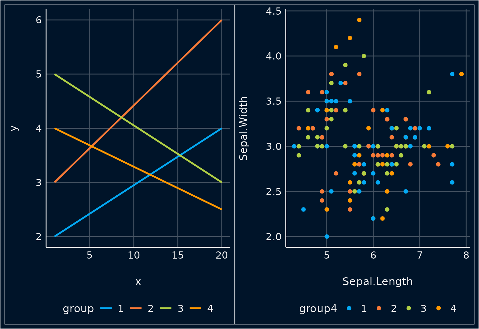
Metro Colors - Five Groups
p1 <- ggplot(d3, aes(x, y, colour = group)) +
  geom_line(linewidth = 1) +
  scale_color_metro(palette = "light")

p2 <- ggplot(iris, aes(Sepal.Length, Sepal.Width, colour = group5)) +
  geom_point2(size = 2.5) +
  scale_color_metro(palette = "light")

plots(p1, p2, n_rows = 1)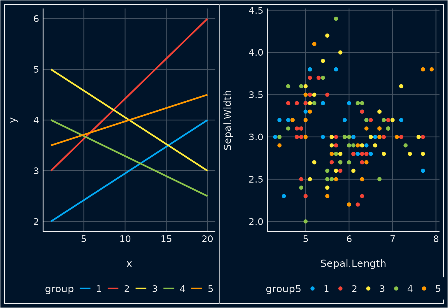
See Colors
See Colors - Three Groups
p1 <- ggplot(d1, aes(x, y, colour = group)) +
  geom_line(linewidth = 1) +
  scale_color_see(palette = "light")

p2 <- ggplot(iris, aes(Sepal.Length, Sepal.Width, colour = Species)) +
  geom_point2(size = 2.5) +
  scale_color_see(palette = "light")

plots(p1, p2, n_rows = 1)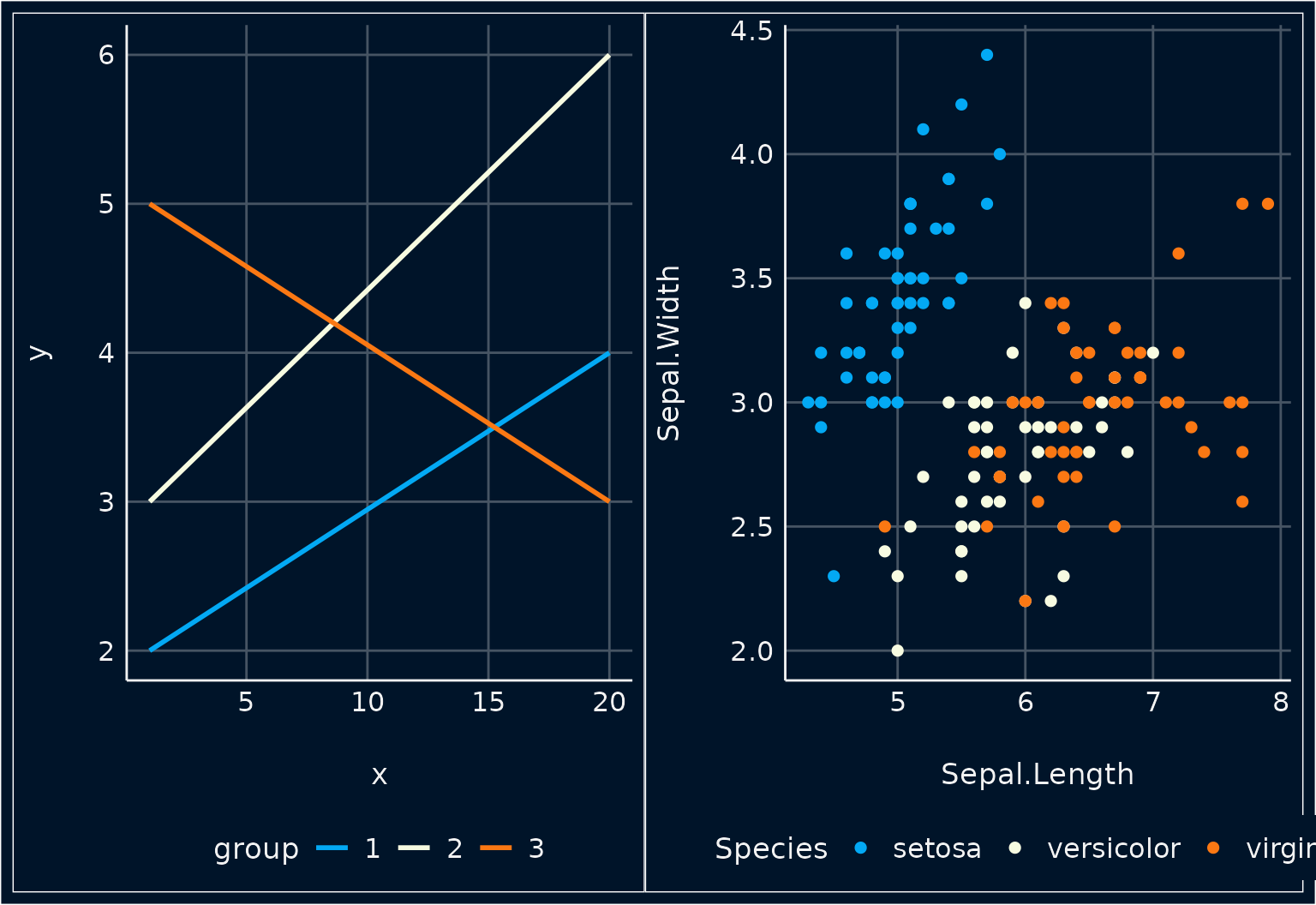
See Colors - Four Groups
p1 <- ggplot(d2, aes(x, y, colour = group)) +
  geom_line(linewidth = 1) +
  scale_color_see(palette = "light")

p2 <- ggplot(iris, aes(Sepal.Length, Sepal.Width, colour = group4)) +
  geom_point2(size = 2.5) +
  scale_color_see(palette = "light")

plots(p1, p2, n_rows = 1)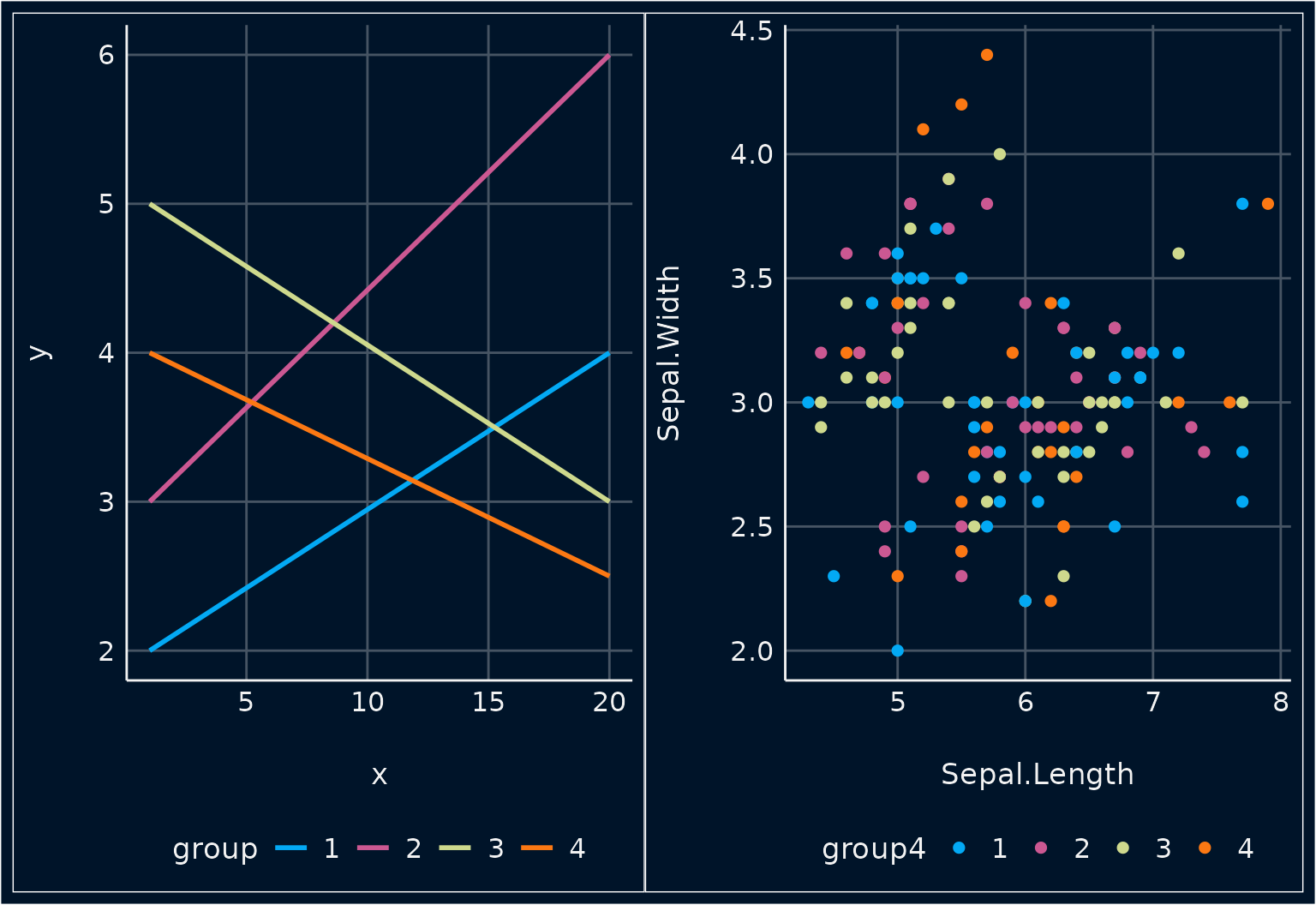
See Colors - Five Groups
p1 <- ggplot(d3, aes(x, y, colour = group)) +
  geom_line(linewidth = 1) +
  scale_color_see(palette = "light")

p2 <- ggplot(iris, aes(Sepal.Length, Sepal.Width, colour = group5)) +
  geom_point2(size = 2.5) +
  scale_color_see(palette = "light")

plots(p1, p2, n_rows = 1)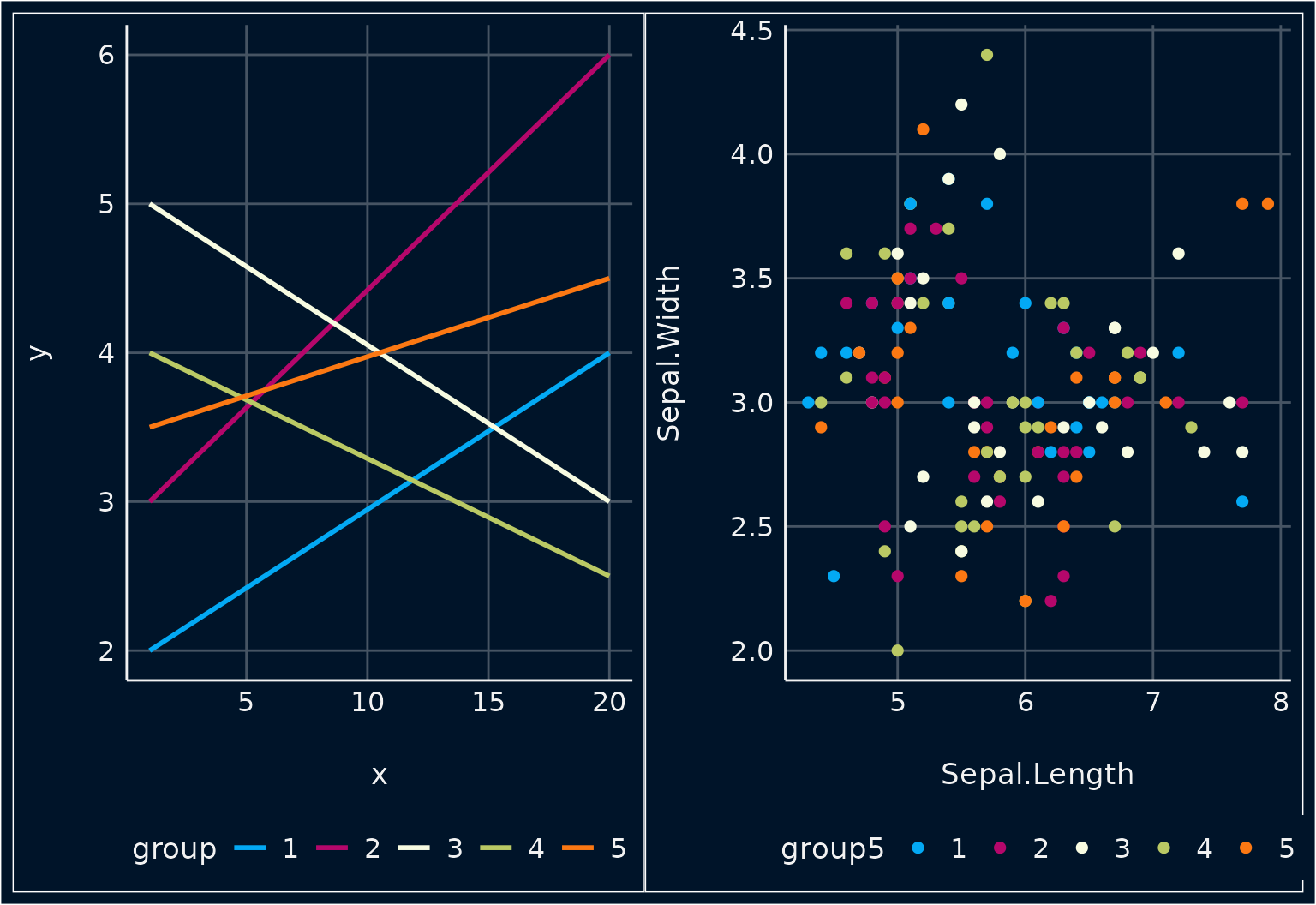
Pizza Colors
Pizza Colors - Three Groups
p1 <- ggplot(d1, aes(x, y, colour = group)) +
  geom_line(linewidth = 1) +
  scale_color_pizza()

p2 <- ggplot(iris, aes(Sepal.Length, Sepal.Width, colour = Species)) +
  geom_point2(size = 2.5) +
  scale_color_pizza()

plots(p1, p2, n_rows = 1)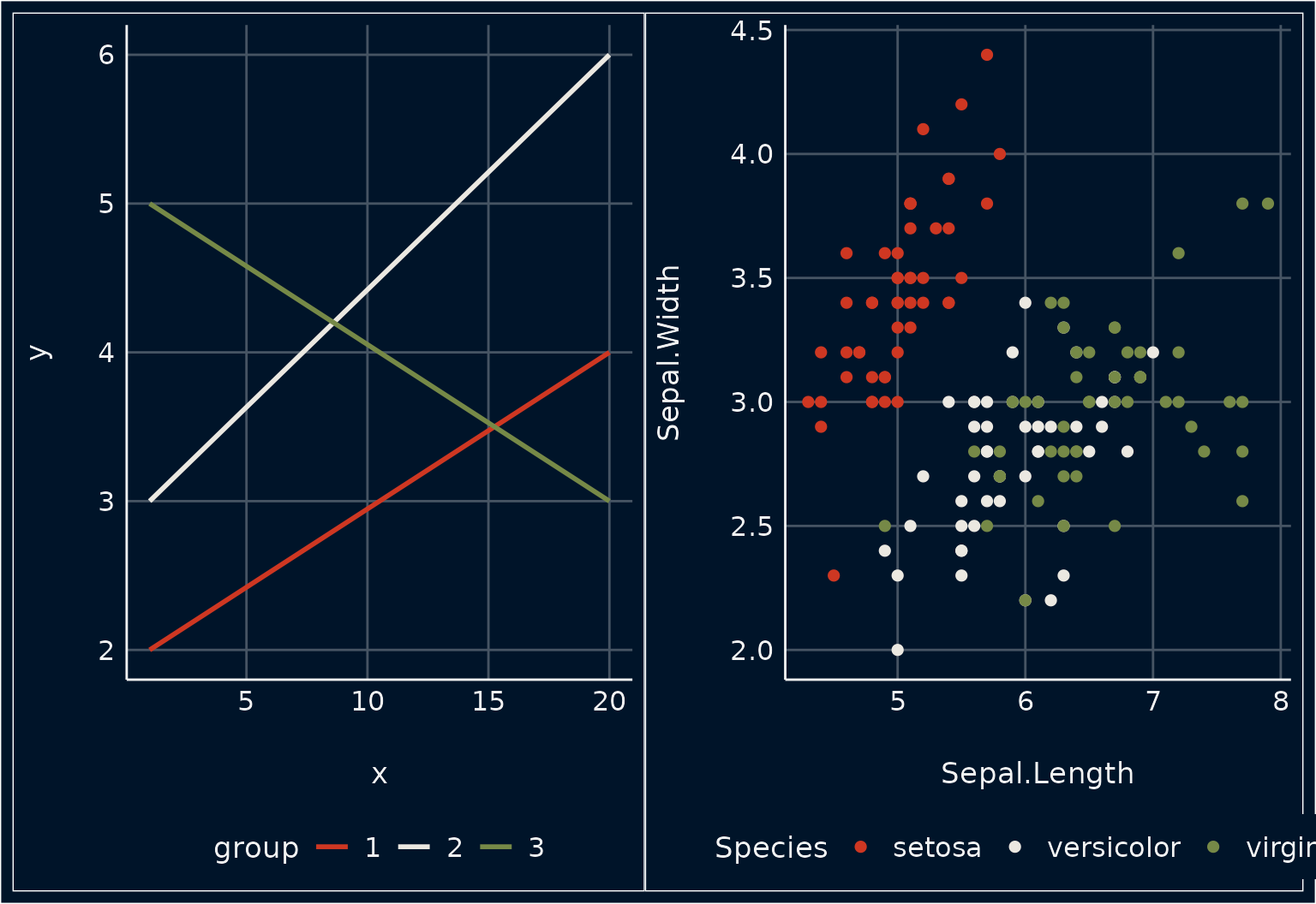
Pizza Colors - Four Groups
p1 <- ggplot(d2, aes(x, y, colour = group)) +
  geom_line(linewidth = 1) +
  scale_color_pizza()

p2 <- ggplot(iris, aes(Sepal.Length, Sepal.Width, colour = group4)) +
  geom_point2(size = 2.5) +
  scale_color_pizza()

plots(p1, p2, n_rows = 1)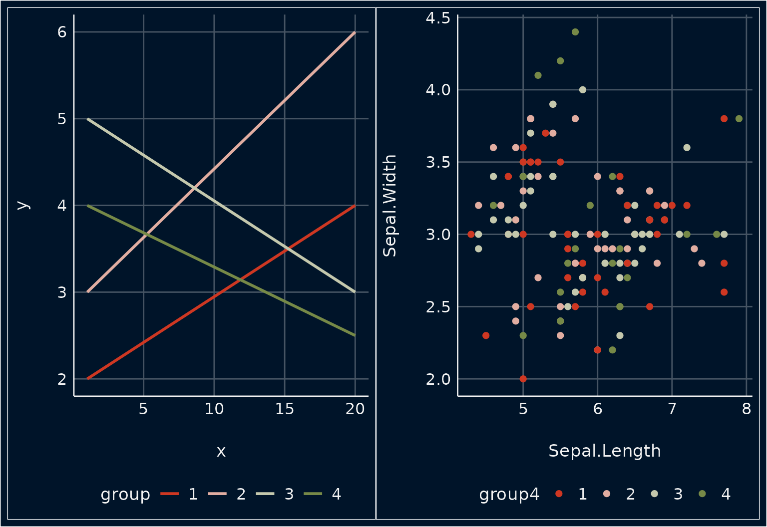
Pizza Colors - Five Groups
p1 <- ggplot(d3, aes(x, y, colour = group)) +
  geom_line(linewidth = 1) +
  scale_color_pizza()

p2 <- ggplot(iris, aes(Sepal.Length, Sepal.Width, colour = group5)) +
  geom_point2(size = 2.5) +
  scale_color_pizza()

plots(p1, p2, n_rows = 1)