Classify the distribution of a model-family using machine learning

Choosing the right distributional family for regression models is essential to get more accurate estimates and standard errors. This function may help to check a models' distributional family and see if the model-family probably should be reconsidered. Since it is difficult to exactly predict the correct model family, consider this function as somewhat experimental.

Usage

check_distribution(model)

Arguments

model

Typically, a model (that should response to residuals()). May also be a numeric vector.

Details

This function uses an internal random forest model to classify the distribution from a model-family. Currently, following distributions are trained (i.e. results of check_distribution() may be one of the following): "bernoulli", "beta", "beta-binomial", "binomial", "cauchy", "chi", "exponential", "F", "gamma", "half-cauchy", "inverse-gamma", "lognormal", "normal", "negative binomial", "negative binomial (zero-inflated)", "pareto", "poisson", "poisson (zero-inflated)", "tweedie", "uniform" and "weibull".

Note the similarity between certain distributions according to shape, skewness, etc. Thus, the predicted distribution may not be perfectly representing the distributional family of the underlying fitted model, or the response value.

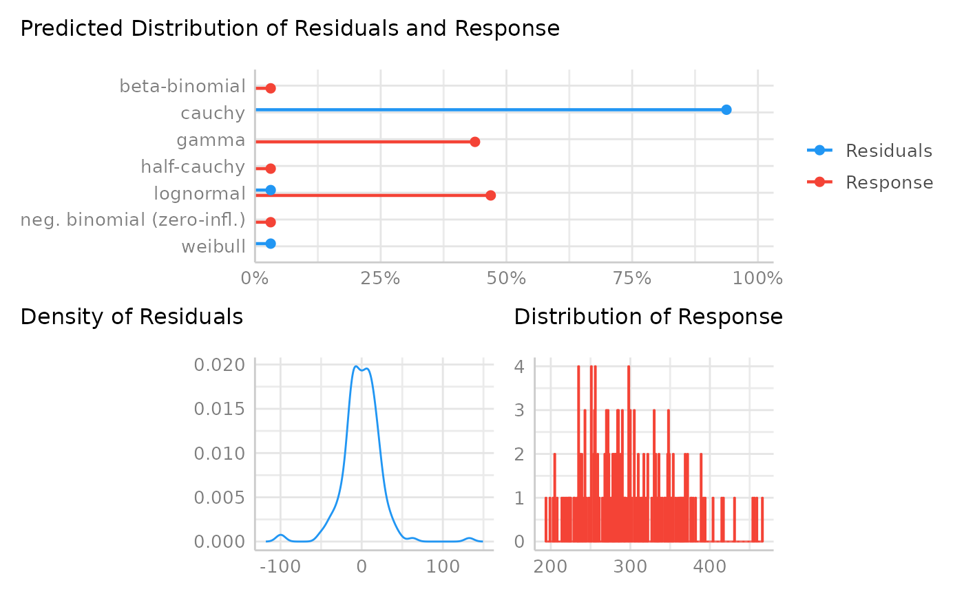
There is a plot() method, which shows the probabilities of all predicted distributions, however, only if the probability is greater than zero.

Note

This function is somewhat experimental and might be improved in future releases. The final decision on the model-family should also be based on theoretical aspects and other information about the data and the model.

There is also a plot()-method implemented in the see-package.

Examples

data(sleepstudy, package = "lme4")
model <<- lme4::lmer(Reaction ~ Days + (Days | Subject), sleepstudy)
check_distribution(model)
#> # Distribution of Model Family
#> 
#> Predicted Distribution of Residuals
#> 
#>                Distribution Probability
#>                      cauchy         91%
#>                       gamma          6%
#>  neg. binomial (zero-infl.)          3%
#> 
#> Predicted Distribution of Response
#> 
#>  Distribution Probability
#>     lognormal         66%
#>         gamma         34%
plot(check_distribution(model))