Binned residuals for binomial logistic regression — binned

Check model quality of binomial logistic regression models.

Usage

binned_residuals(
  model,
  term = NULL,
  n_bins = NULL,
  show_dots = NULL,
  ci = 0.95,
  ci_type = "exact",
  residuals = "deviance",
  iterations = 1000,
  verbose = TRUE,
  ...
)

Arguments

model: A glm-object with binomial-family.
term: Name of independent variable from x. If not NULL, average residuals for the categories of term are plotted; else, average residuals for the estimated probabilities of the response are plotted.
n_bins: Numeric, the number of bins to divide the data. If n_bins = NULL, the square root of the number of observations is taken.
show_dots: Logical, if TRUE, will show data points in the plot. Set to FALSE for models with many observations, if generating the plot is too time-consuming. By default, show_dots = NULL. In this case binned_residuals() tries to guess whether performance will be poor due to a very large model and thus automatically shows or hides dots.
ci: Numeric, the confidence level for the error bounds.
ci_type: Character, the type of error bounds to calculate. Can be "exact" (default), "gaussian" or "boot". "exact" calculates the error bounds based on the exact binomial distribution, using binom.test(). "gaussian" uses the Gaussian approximation, while "boot" uses a simple bootstrap method, where confidence intervals are calculated based on the quantiles of the bootstrap distribution.
residuals: Character, the type of residuals to calculate. Can be "deviance" (default), "pearson" or "response". It is recommended to use "response" only for those models where other residuals are not available.
iterations: Integer, the number of iterations to use for the bootstrap method. Only used if ci_type = "boot".
verbose: Toggle warnings and messages.
...: Currently not used.

Value

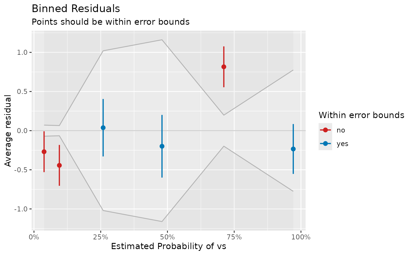
A data frame representing the data that is mapped in the accompanying plot. In case all residuals are inside the error bounds, points are black. If some of the residuals are outside the error bounds (indicated by the grey-shaded area), blue points indicate residuals that are OK, while red points indicate model under- or over-fitting for the relevant range of estimated probabilities.

Details

Binned residual plots are achieved by "dividing the data into categories (bins) based on their fitted values, and then plotting the average residual versus the average fitted value for each bin." (Gelman, Hill 2007: 97). If the model were true, one would expect about 95% of the residuals to fall inside the error bounds.

If term is not NULL, one can compare the residuals in relation to a specific model predictor. This may be helpful to check if a term would fit better when transformed, e.g. a rising and falling pattern of residuals along the x-axis is a signal to consider taking the logarithm of the predictor (cf. Gelman and Hill 2007, pp. 97-98).

Note

binned_residuals() returns a data frame, however, the print() method only returns a short summary of the result. The data frame itself is used for plotting. The plot() method, in turn, creates a ggplot-object.

References

Gelman, A., and Hill, J. (2007). Data analysis using regression and multilevel/hierarchical models. Cambridge; New York: Cambridge University Press.

Examples

model <- glm(vs ~ wt + mpg, data = mtcars, family = "binomial")
result <- binned_residuals(model)
result
#> Warning: Probably bad model fit. Only about 50% of the residuals are inside the error bounds.
#> 

# look at the data frame
as.data.frame(result)
#>                 xbar        ybar n       x.lo       x.hi         se     CI_low
#> conf_int  0.03786483 -0.26905395 5 0.01744776 0.06917366 0.07079661 -0.5299658
#> conf_int1 0.09514191 -0.44334345 5 0.07087498 0.15160143 0.06530245 -0.7042553
#> conf_int2 0.25910531  0.03762945 6 0.17159955 0.35374001 1.02017708 -0.3293456
#> conf_int3 0.47954643 -0.19916717 5 0.38363314 0.54063600 1.16107852 -0.5994783
#> conf_int4 0.71108931  0.81563262 5 0.57299903 0.89141359 0.19814385  0.5547207
#> conf_int5 0.97119262 -0.23399465 6 0.91147360 0.99815623 0.77513642 -0.5525066
#>                CI_high group
#> conf_int  -0.008142076    no
#> conf_int1 -0.182431572    no
#> conf_int2  0.404604465   yes
#> conf_int3  0.201143953   yes
#> conf_int4  1.076544495    no
#> conf_int5  0.084517267   yes

# \donttest{
# plot
plot(result, show_dots = TRUE)

# }