Compare, Test, and Select Models

Comparing vs. Testing

Let’s imagine that we are interested in explaining the variability in the Sepal.Length using 3 different predictors. For that, we can build 3 linear models.

model1 <- lm(Sepal.Length ~ Petal.Length, data = iris)
model2 <- lm(Sepal.Length ~ Petal.Width, data = iris)
model3 <- lm(Sepal.Length ~ Sepal.Width, data = iris)

Comparing Indices of Model Performance

The eponymous function from the package, performance(), can be used to compute different indices of performance (an umbrella term for indices of fit).

library(performance)
library(insight)

# we will use `print_md` function to display a well-formatted table
result <- performance(model1)
print_md(result)

Indices of model performance

AIC	AICc	BIC	R2	R2 (adj.)	RMSE	Sigma
160.04	160.20	169.07	0.76	0.76	0.40	0.41

But for multiple models, one can obtain a useful table to compare these indices at a glance using the compare_performance() function.

result <- compare_performance(model1, model2, model3)
print_md(result)

Comparison of Model Performance Indices

Name	Model	AIC (weights)	AICc (weights)	BIC (weights)	R2	R2 (adj.)	RMSE	Sigma
model1	lm	160.0 (>.999)	160.2 (>.999)	169.1 (>.999)	0.76	0.76	0.40	0.41
model2	lm	208.2 (<.001)	208.4 (<.001)	217.3 (<.001)	0.67	0.67	0.47	0.48
model3	lm	372.0 (<.001)	372.2 (<.001)	381.0 (<.001)	0.01	7.16e-03	0.82	0.83

If you remember your stats lessons, while comparing different model fits, you would like to choose a model that has a high R^2 value (a measure of how much variance is explained by predictors), low AIC and BIC values, and low root mean squared error (RMSE). Based on these criteria, we can immediately see that model1 has the best fit.

If you don’t like looking at tables, you can also plot them using a plotting method supported in see package:

library(see)

plot(compare_performance(model1, model2, model3))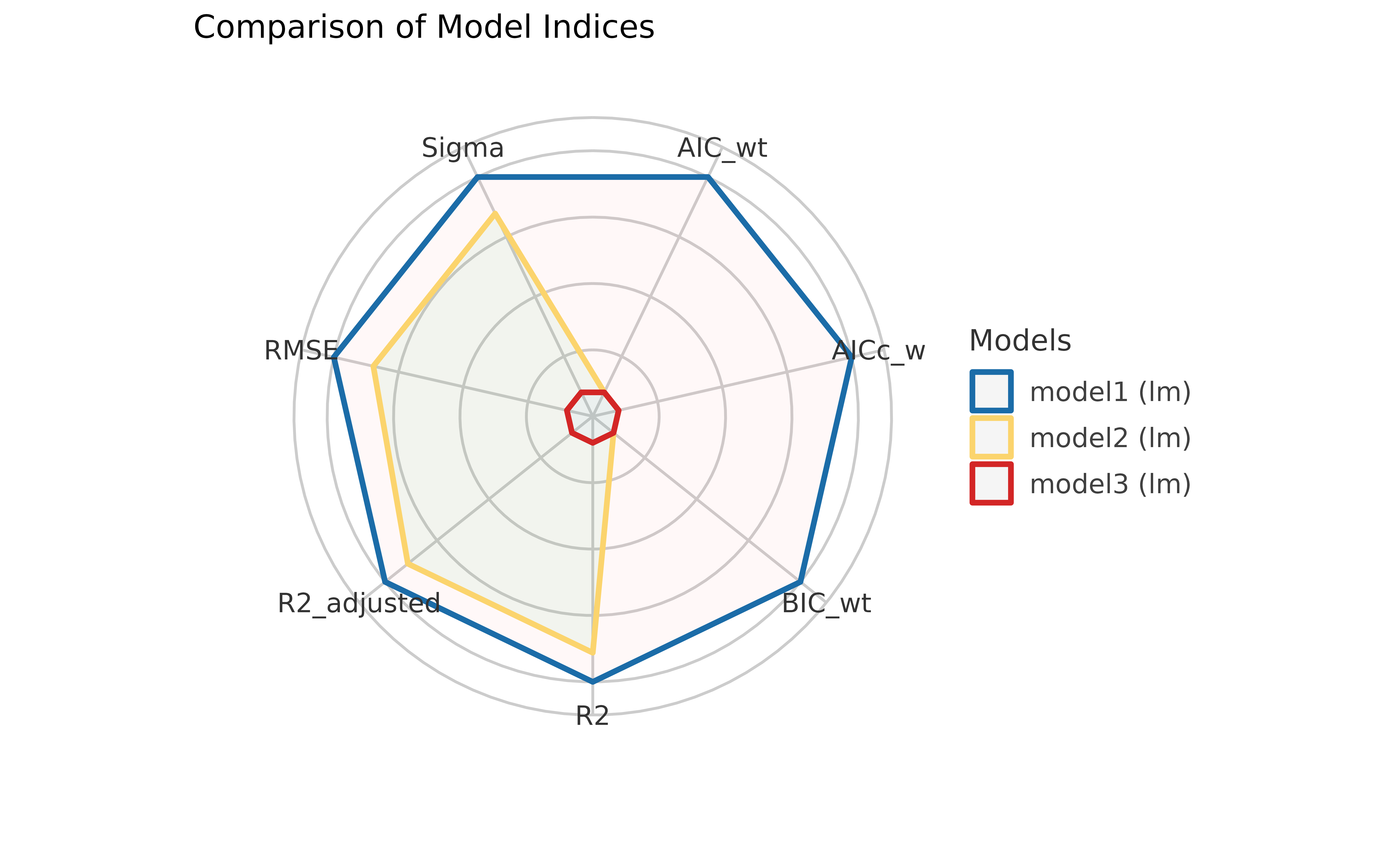

For more, see: https://easystats.github.io/see/articles/performance.html

Testing Models

While comparing these indices is often useful, making a decision (for instance, which model to keep or drop) can often be hard, as the indices can give conflicting suggestions. Additionally, it is sometimes unclear which index to favour in the given context.

This is one of the reason why tests are useful, as they facilitate decisions via (infamous) “significance” indices, like p-values (in frequentist framework) or Bayes Factors (in Bayesian framework).

result <- test_performance(model1, model2, model3)
print_md(result)

Name	Model	BF	Omega2	p (Omega2)	LR	p (LR)
model1	lm
model2	lm	< 0.001	0.19	< .001	4.57	< .001
model3	lm	< 0.001	0.56	< .001	11.52	< .001

Each model is compared to model1.

However, these tests also have strong limitations and shortcomings, and cannot be used as the one criterion to rule them all!

You can find more information on how these tests here.

Experimenting

Although we have shown here examples only with simple linear models, we will highly encourage you to try these functions out with models of your choosing. For example, these functions work with mixed-effects regression models, Bayesian regression models, etc.

To demonstrate this, we will run Bayesian versions of linear regression models we just compared:

library(rstanarm)

model1 <- stan_glm(Sepal.Length ~ Petal.Length, data = iris, refresh = 0)
model2 <- stan_glm(Sepal.Length ~ Petal.Width, data = iris, refresh = 0)
model3 <- stan_glm(Sepal.Length ~ Sepal.Width, data = iris, refresh = 0)

result <- compare_performance(model1, model2, model3)
print_md(result)

Comparison of Model Performance Indices

Name	Model	ELPD	ELPD_SE	LOOIC (weights)	LOOIC_SE	WAIC (weights)	R2	R2 (adj.)	RMSE	Sigma
model1	stanreg	-80.02	8.35	160.0 (>.999)	16.70	160.0 (>.999)	0.76	0.76	0.40	0.41
model2	stanreg	-104.22	9.26	208.4 (<.001)	18.52	208.4 (<.001)	0.67	0.66	0.47	0.48
model3	stanreg	-185.70	7.88	371.4 (<.001)	15.76	371.4 (<.001)	0.01	-1.71e-03	0.82	0.83

Note that, since these are Bayesian regression models, the function automatically picked up the appropriate indices to compare!

If you are unfamiliar with some of these, explore more here.

Now it’s your turn to play! :)