Reuse of this Material
Note: This vignette is an extended write-up of the Behavior Research Methods paper. This educational module can be freely reused for teaching purposes as long as the original BRM paper is cited. The raw code file, which can be adapted to other rmarkdown formats for teaching purposes, can be accessed here. To contribute to and improve this content directly, please submit a Pull Request at the {performance} package GitHub repository by following our usual contributing guidelines: https://easystats.github.io/performance/CONTRIBUTING.html. To report issues or problems, with this module, or seek support, please open an issue: https://github.com/easystats/performance/issues.
Reference:
Thériault, R., Ben-Shachar, M. S., Patil, I., Lüdecke, D., Wiernik, B. M., & Makowski, D. (2024). Check your outliers! An introduction to identifying statistical outliers in R with easystats. Behavior Research Methods, 1-11. https://doi.org/10.3758/s13428-024-02356-w
Summary
Beyond the challenge of keeping up-to-date with current best practices regarding the diagnosis and treatment of outliers, an additional difficulty arises concerning the mathematical implementation of the recommended methods. In this vignette, we provide an overview of current recommendations and best practices and demonstrate how they can easily and conveniently be implemented in the R statistical computing software, using the {performance} package of the easystats ecosystem. We cover univariate, multivariate, and model-based statistical outlier detection methods, their recommended threshold, standard output, and plotting methods. We conclude with recommendations on the handling of outliers: the different theoretical types of outliers, whether to exclude or winsorize them, and the importance of transparency.
Statement of Need
Real-life data often contain observations that can be considered abnormal when compared to the main population. The cause of it—be it because they belong to a different distribution (originating from a different generative process) or simply being extreme cases, statistically rare but not impossible—can be hard to assess, and the boundaries of “abnormal” difficult to define.
Nonetheless, the improper handling of these outliers can substantially affect statistical model estimations, biasing effect estimations and weakening the models’ predictive performance. It is thus essential to address this problem in a thoughtful manner. Yet, despite the existence of established recommendations and guidelines, many researchers still do not treat outliers in a consistent manner, or do so using inappropriate strategies (Simmons et al. 2011; Leys et al. 2013).
One possible reason is that researchers are not aware of the existing recommendations, or do not know how to implement them using their analysis software. In this paper, we show how to follow current best practices for automatic and reproducible statistical outlier detection (SOD) using R and the {performance} package (Lüdecke et al. 2021), which is part of the easystats ecosystem of packages that build an R framework for easy statistical modeling, visualization, and reporting (Lüdecke et al. [2019] 2023). Installation instructions can be found on GitHub or its website, and its list of dependencies on CRAN.
The instructional materials that follow are aimed at an audience of researchers who want to follow good practices, and are appropriate for advanced undergraduate students, graduate students, professors, or professionals having to deal with the nuances of outlier treatment.
Identifying Outliers
Although many researchers attempt to identify outliers with measures based on the mean (e.g., z scores), those methods are problematic because the mean and standard deviation themselves are not robust to the influence of outliers and those methods also assume normally distributed data (i.e., a Gaussian distribution). Therefore, current guidelines recommend using robust methods to identify outliers, such as those relying on the median as opposed to the mean (Leys et al. 2019, 2013, 2018).
Nonetheless, which exact outlier method to use depends on many factors. In some cases, eye-gauging odd observations can be an appropriate solution, though many researchers will favour algorithmic solutions to detect potential outliers, for example, based on a continuous value expressing the observation stands out from the others.
One of the factors to consider when selecting an algorithmic outlier detection method is the statistical test of interest. When using a regression model, relevant information can be found by identifying observations that do not fit well with the model. This approach, known as model-based outliers detection (as outliers are extracted after the statistical model has been fit), can be contrasted with distribution-based outliers detection, which is based on the distance between an observation and the “center” of its population. Various quantification strategies of this distance exist for the latter, both univariate (involving only one variable at a time) or multivariate (involving multiple variables).
When no method is readily available to detect model-based outliers, such as for structural equation modelling (SEM), looking for multivariate outliers may be of relevance. For simple tests (t tests or correlations) that compare values of the same variable, it can be appropriate to check for univariate outliers. However, univariate methods can give false positives since t tests and correlations, ultimately, are also models/multivariable statistics. They are in this sense more limited, but we show them nonetheless for educational purposes.
Importantly, whatever approach researchers choose remains a subjective decision, which usage (and rationale) must be transparently documented and reproducible (Leys et al. 2019). Researchers should commit (ideally in a preregistration) to an outlier treatment method before collecting the data. They should report in the paper their decisions and details of their methods, as well as any deviation from their original plan. These transparency practices can help reduce false positives due to excessive researchers’ degrees of freedom (i.e., choice flexibility throughout the analysis). In the following section, we will go through each of the mentioned methods and provide examples on how to implement them with R.
Univariate Outliers
Researchers frequently attempt to identify outliers using measures of deviation from the center of a variable’s distribution. One of the most popular such procedure is the z score transformation, which computes the distance in standard deviation (SD) from the mean. However, as mentioned earlier, this popular method is not robust. Therefore, for univariate outliers, it is recommended to use the median along with the Median Absolute Deviation (MAD), which are more robust than the interquartile range or the mean and its standard deviation (Leys et al. 2019, 2013).
Researchers can identify outliers based on robust (i.e., MAD-based)
z scores using the check_outliers() function of
the {performance} package, by specifying
method = "zscore_robust".1 Although Leys et al. (2013) suggest a default threshold
of 2.5 and Leys et al. (2019) a threshold
of 3, {performance} uses by default a less conservative
threshold of ~3.29.2 That is, data points will be flagged as
outliers if they go beyond +/- ~3.29 MAD. Users can adjust this
threshold using the threshold argument.
Below we provide example code using the mtcars dataset,
which was extracted from the 1974 Motor Trend US magazine. The
dataset contains fuel consumption and 10 characteristics of automobile
design and performance for 32 different car models (see
?mtcars for details). We chose this dataset because it is
accessible from base R and familiar to many R users. We might want to
conduct specific statistical analyses on this data set, say, t
tests or structural equation modelling, but first, we want to check for
outliers that may influence those test results.
Because the automobile names are stored as column names in
mtcars, we first have to convert them to an ID column to
benefit from the check_outliers() ID argument. Furthermore,
we only really need a couple columns for this demonstration, so we
choose the first four (mpg = Miles/(US) gallon;
cyl = Number of cylinders; disp =
Displacement; hp = Gross horsepower). Finally, because
there are no outliers in this dataset, we add two artificial outliers
before running our function.
library(performance)

# Create some artificial outliers and an ID column
data <- rbind(mtcars[1:4], 42, 55)
data <- cbind(car = row.names(data), data)

outliers <- check_outliers(data, method = "zscore_robust", ID = "car")
outliers
> 2 outliers detected: cases 33, 34.
> - Based on the following method and threshold: zscore_robust (3.291).
> - For variables: mpg, cyl, disp, hp.
>
> -----------------------------------------------------------------------------
>
> The following observations were considered outliers for two or more
> variables by at least one of the selected methods:
>
> Row car n_Zscore_robust
> 1 33 33 2
> 2 34 34 2
>
> -----------------------------------------------------------------------------
> Outliers per variable (zscore_robust):
>
> $mpg
> Row car Distance_Zscore_robust
> 33 33 33 3.7
> 34 34 34 5.8
>
> $cyl
> Row car Distance_Zscore_robust
> 33 33 33 12
> 34 34 34 17What we see is that check_outliers() with the robust
z score method detected two outliers: cases 33 and 34, which
were the observations we added ourselves. They were flagged for two
variables specifically: mpg (Miles/(US) gallon) and
cyl (Number of cylinders), and the output provides their
exact z score for those variables.
We describe how to deal with those cases in more details later in the
paper, but should we want to exclude these detected outliers from the
main dataset, we can extract row numbers using which() on
the output object, which can then be used for indexing:
which(outliers)> [1] 33 34
data_clean <- data[-which(outliers), ]All check_outliers() output objects possess a
plot() method, meaning it is also possible to visualize the
outliers using the generic plot() function on the resulting
outlier object after loading the {see} package.
> $threshold_outliers
> [1] 33 34
>
> $threshold
> [1] 3.3
>
> $elbow_outliers
> [1] 33 34
>
> $elbow_threshold
> [1] 9.5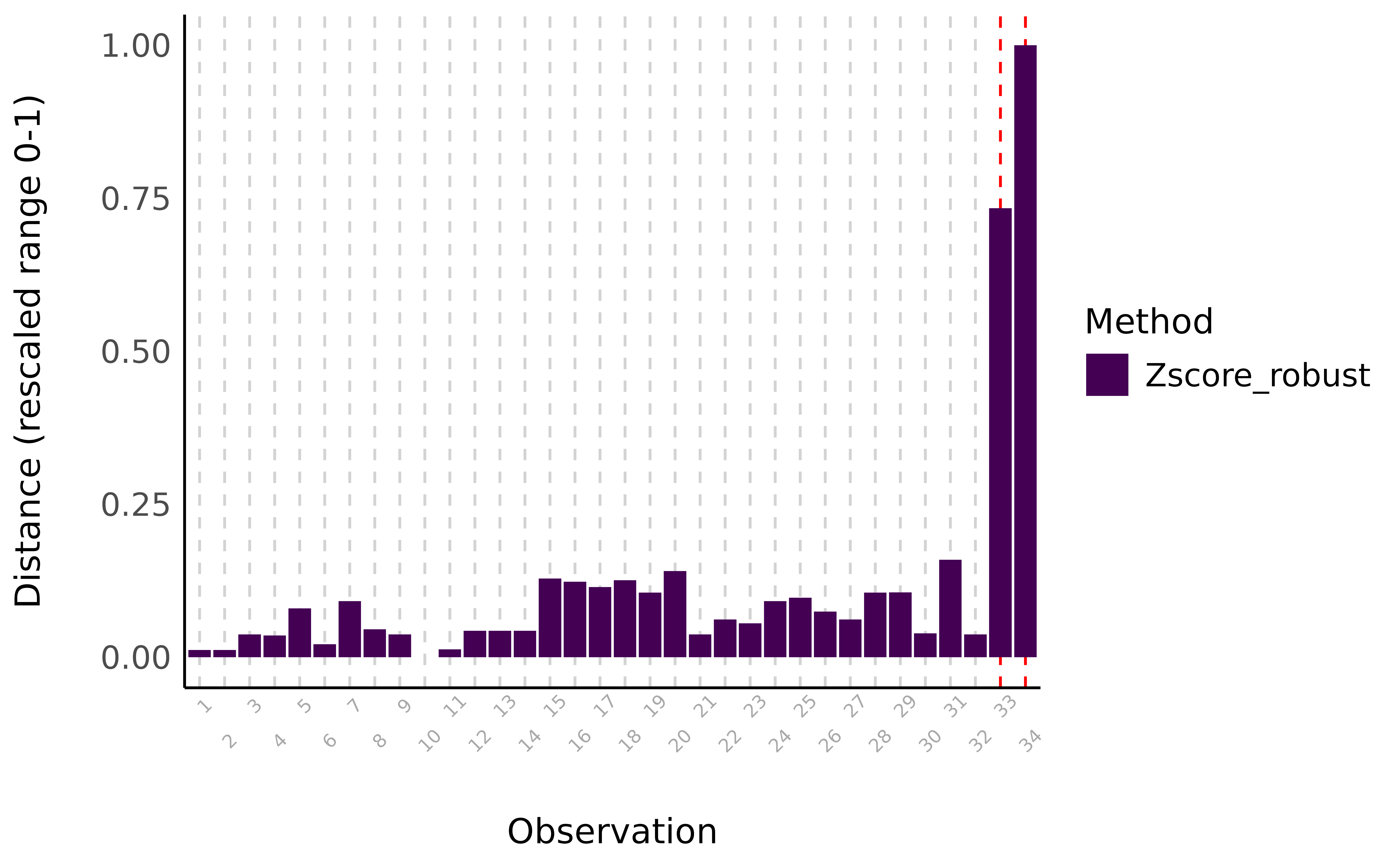
Visual depiction of outliers using the robust z-score method. The distance represents an aggregate score for variables mpg, cyl, disp, and hp.
Other univariate methods are available, such as using the interquartile range (IQR), or based on different intervals, such as the Highest Density Interval (HDI) or the Bias Corrected and Accelerated Interval (BCI). These methods are documented and described in the function’s help page.
Multivariate Outliers
Univariate outliers can be useful when the focus is on a particular variable, for instance the reaction time, as extreme values might be indicative of inattention or non-task-related behavior3.
However, in many scenarios, variables of a data set are not independent, and an abnormal observation will impact multiple dimensions. For instance, a participant giving random answers to a questionnaire. In this case, computing the z score for each of the questions might not lead to satisfactory results. Instead, one might want to look at these variables together.
One common approach for this is to compute multivariate distance metrics such as the Mahalanobis distance. Although the Mahalanobis distance is very popular, just like the regular z scores method, it is not robust and is heavily influenced by the outliers themselves. Therefore, for multivariate outliers, it is recommended to use the Minimum Covariance Determinant, a robust version of the Mahalanobis distance (MCD, Leys et al. 2018, 2019).
In {performance}’s check_outliers(), one can
use this approach with method = "mcd".4
outliers <- check_outliers(data, method = "mcd", verbose = FALSE)
outliers
> 2 outliers detected: cases 33, 34.
> - Based on the following method and threshold: mcd (20).
> - For variables: mpg, cyl, disp, hp.Here, we detected 9 multivariate outliers (i.e,. when looking at all variables of our dataset together).
plot(outliers)> $threshold_outliers
> [1] 33 34
>
> $threshold
> [1] 18
>
> $elbow_outliers
> [1] 33 34
>
> $elbow_threshold
> [1] 3547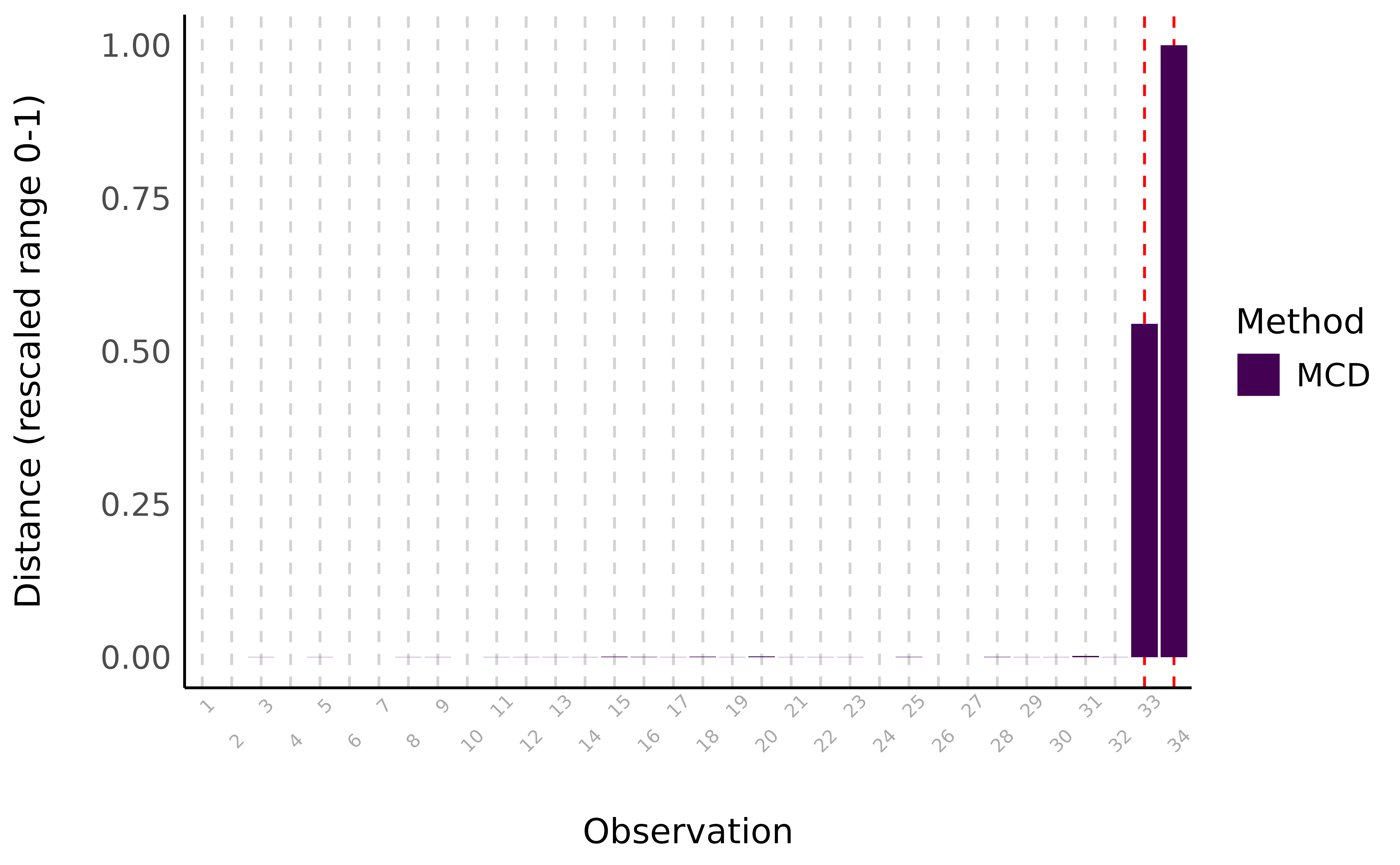
Visual depiction of outliers using the Minimum Covariance Determinant (MCD) method, a robust version of the Mahalanobis distance. The distance represents the MCD scores for variables mpg, cyl, disp, and hp.
Other multivariate methods are available, such as another type of robust Mahalanobis distance that in this case relies on an orthogonalized Gnanadesikan-Kettenring pairwise estimator (Gnanadesikan and Kettenring 1972). These methods are documented and described in the function’s help page.
Model-Based Outliers
Working with regression models creates the possibility of using model-based SOD methods. These methods rely on the concept of leverage, that is, how much influence a given observation can have on the model estimates. If few observations have a relatively strong leverage/influence on the model, one can suspect that the model’s estimates are biased by these observations, in which case flagging them as outliers could prove helpful (see next section, “Handling Outliers”).
In {performance}, two such model-based SOD methods are currently
available: Cook’s distance, for regular regression models, and Pareto,
for Bayesian models. As such, check_outliers() can be
applied directly on regression model objects, by simply specifying
method = "cook" (or method = "pareto" for
Bayesian models).5
Currently, most lm models are supported (with the exception of
glmmTMB, lmrob, and glmrob
models), as long as they are supported by the underlying functions
stats::cooks.distance() (or
loo::pareto_k_values()) and
insight::get_data() (for a full list of the 225 models
currently supported by the insight package, see https://easystats.github.io/insight/#list-of-supported-models-by-class).
Also note that although check_outliers() supports the pipe
operators (|> or %>%), it does not
support tidymodels at this time. We show a demo below.
model <- lm(disp ~ mpg * hp, data = data)
outliers <- check_outliers(model, method = "cook")
outliers
> 2 outliers detected: cases 31, 34.
> - Based on the following method and threshold: cook (0.806).
> - For variable: (Whole model).
plot(outliers)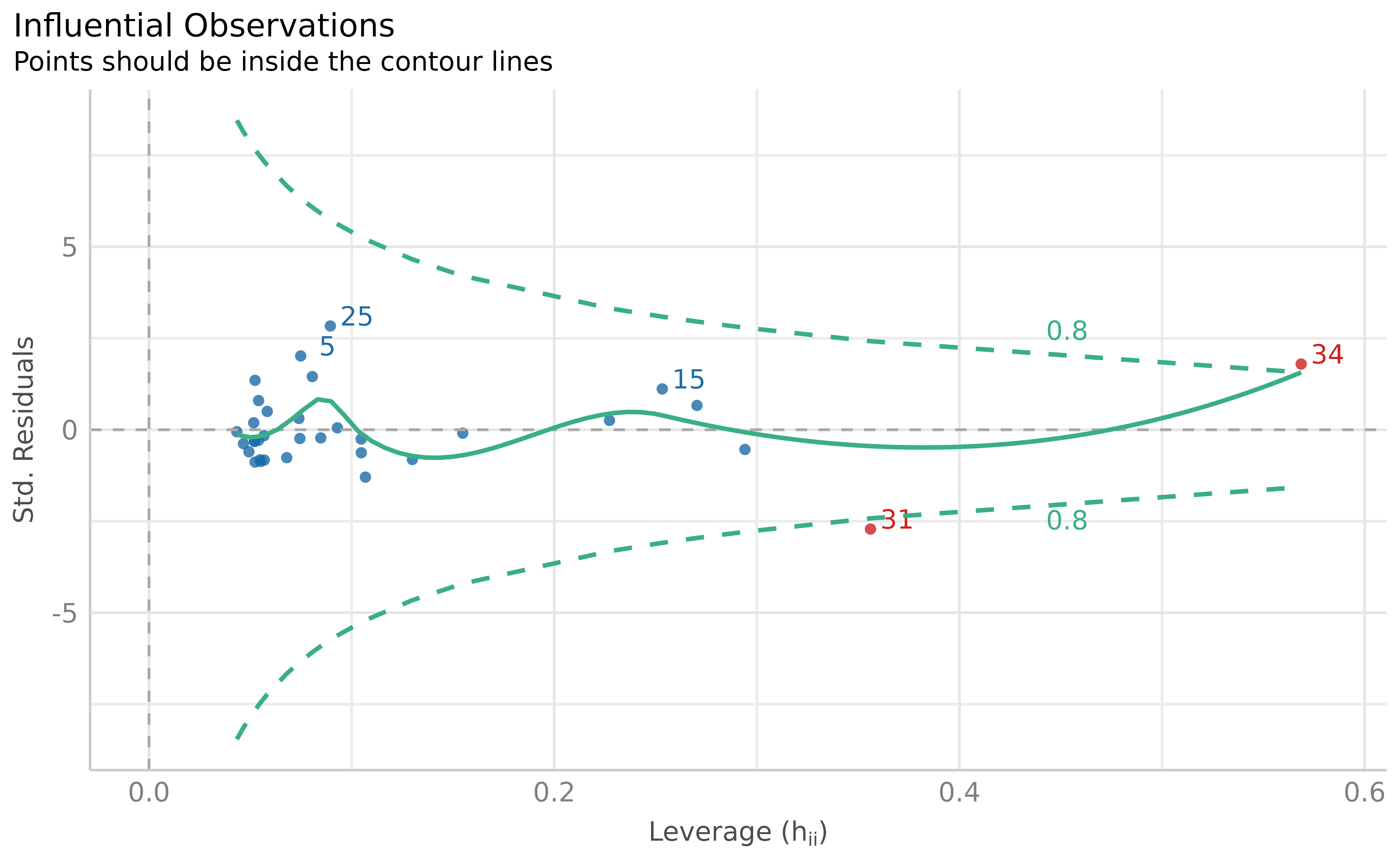
Visual depiction of outliers based on Cook’s distance (leverage and standardized residuals), based on the fitted model.
Using the model-based outlier detection method, we identified two outliers.
Table 1 below summarizes which methods to use in which cases, and with what threshold. The recommended thresholds are the default thresholds.
Table 1
Summary of Statistical Outlier Detection Methods Recommendations
Statistical Test |
Diagnosis Method |
Recommended Threshold |
Function Usage |
|---|---|---|---|
Supported regression model |
Model-based: Cook (or Pareto for Bayesian models) |
qf(0.5, ncol(x), nrow(x) - ncol(x)) (or 0.7 for Pareto) |
check_outliers(model, method = “cook”) |
Structural Equation Modeling (or other unsupported model) |
Multivariate: Minimum Covariance Determinant (MCD) |
qchisq(p = 1 - 0.001, df = ncol(x)) |
check_outliers(data, method = “mcd”) |
Simple test with few variables (t test, correlation, etc.) |
Univariate: robust z scores (MAD) |
qnorm(p = 1 - 0.001 / 2), ~ 3.29 |
check_outliers(data, method = “zscore_robust”) |
Cook’s Distance vs. MCD
Leys et al. (2018) report a preference for the MCD method over Cook’s distance. This is because Cook’s distance removes one observation at a time and checks its corresponding influence on the model each time (Cook 1977), and flags any observation that has a large influence. In the view of these authors, when there are several outliers, the process of removing a single outlier at a time is problematic as the model remains “contaminated” or influenced by other possible outliers in the model, rendering this method suboptimal in the presence of multiple outliers.
However, distribution-based approaches are not a silver bullet
either, and there are cases where the usage of methods agnostic to
theoretical and statistical models of interest might be problematic. For
example, a very tall person would be expected to also be much heavier
than average, but that would still fit with the expected association
between height and weight (i.e., it would be in line with a model such
as weight ~ height). In contrast, using multivariate
outlier detection methods there may flag this person as being an
outlier—being unusual on two variables, height and weight—even though
the pattern fits perfectly with our predictions.
In the example below, we plot the raw data and see two possible outliers. The first one falls along the regression line, and is therefore “in line” with our hypothesis. The second one clearly diverges from the regression line, and therefore we can conclude that this outlier may have a disproportionate influence on our model.
data <- women[rep(seq_len(nrow(women)), each = 100), ]
data <- rbind(data, c(100, 258), c(100, 200))
model <- lm(weight ~ height, data)
rempsyc::nice_scatter(data, "height", "weight")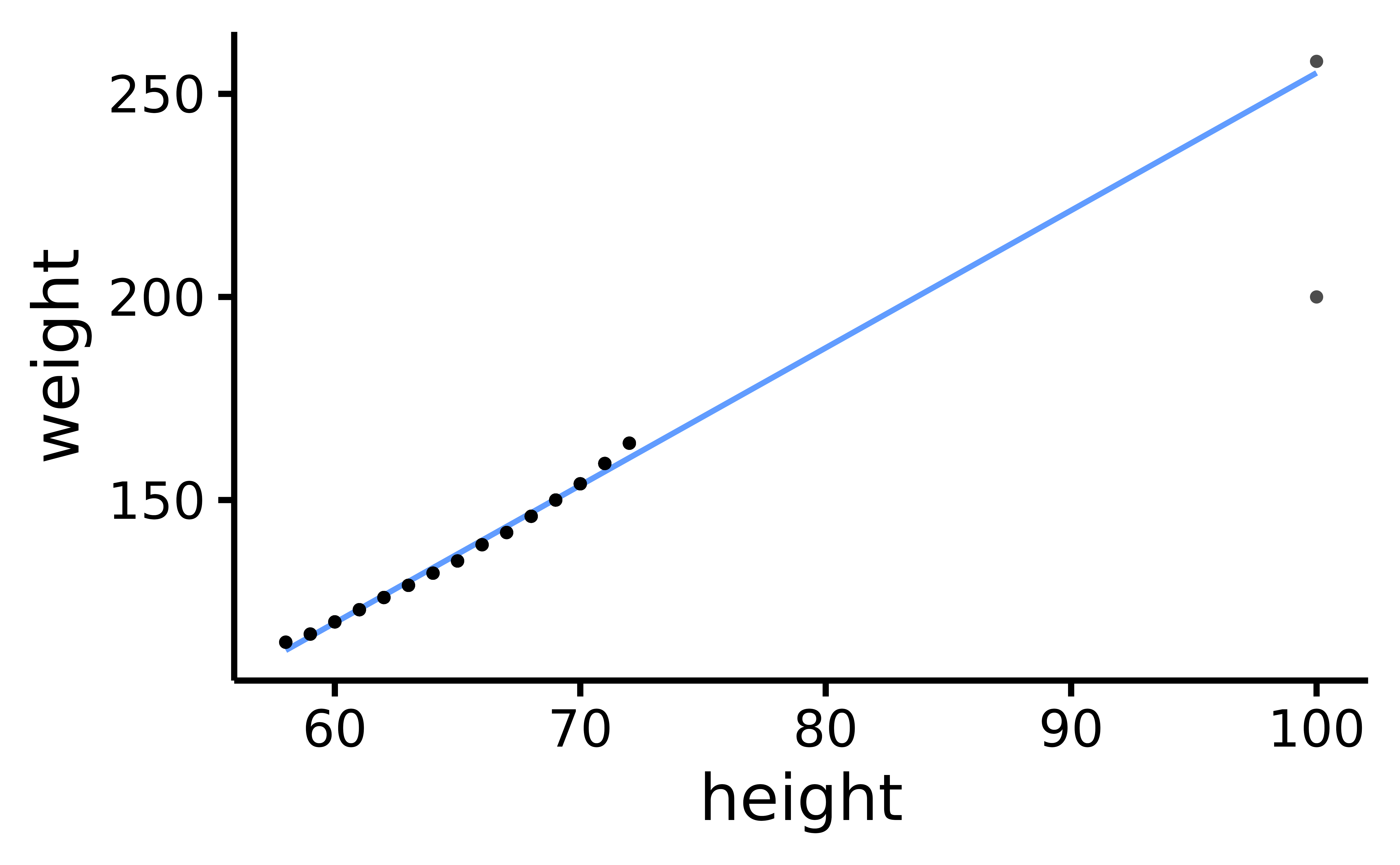
Scatter plot of height and weight, with two extreme observations: one model-consistent (top-right) and the other, model-inconsistent (i.e., an outlier; bottom-right).
Using either the z-score or MCD methods, our model-consistent observation will be incorrectly flagged as an outlier or influential observation.
outliers <- check_outliers(model, method = c("zscore_robust", "mcd"), verbose = FALSE)
which(outliers)
> [1] 1501 1502In contrast, the model-based detection method displays the desired behaviour: it correctly flags the person who is very tall but very light, without flagging the person who is both tall and heavy.
outliers <- check_outliers(model, method = "cook")
which(outliers)
> [1] 1502
plot(outliers)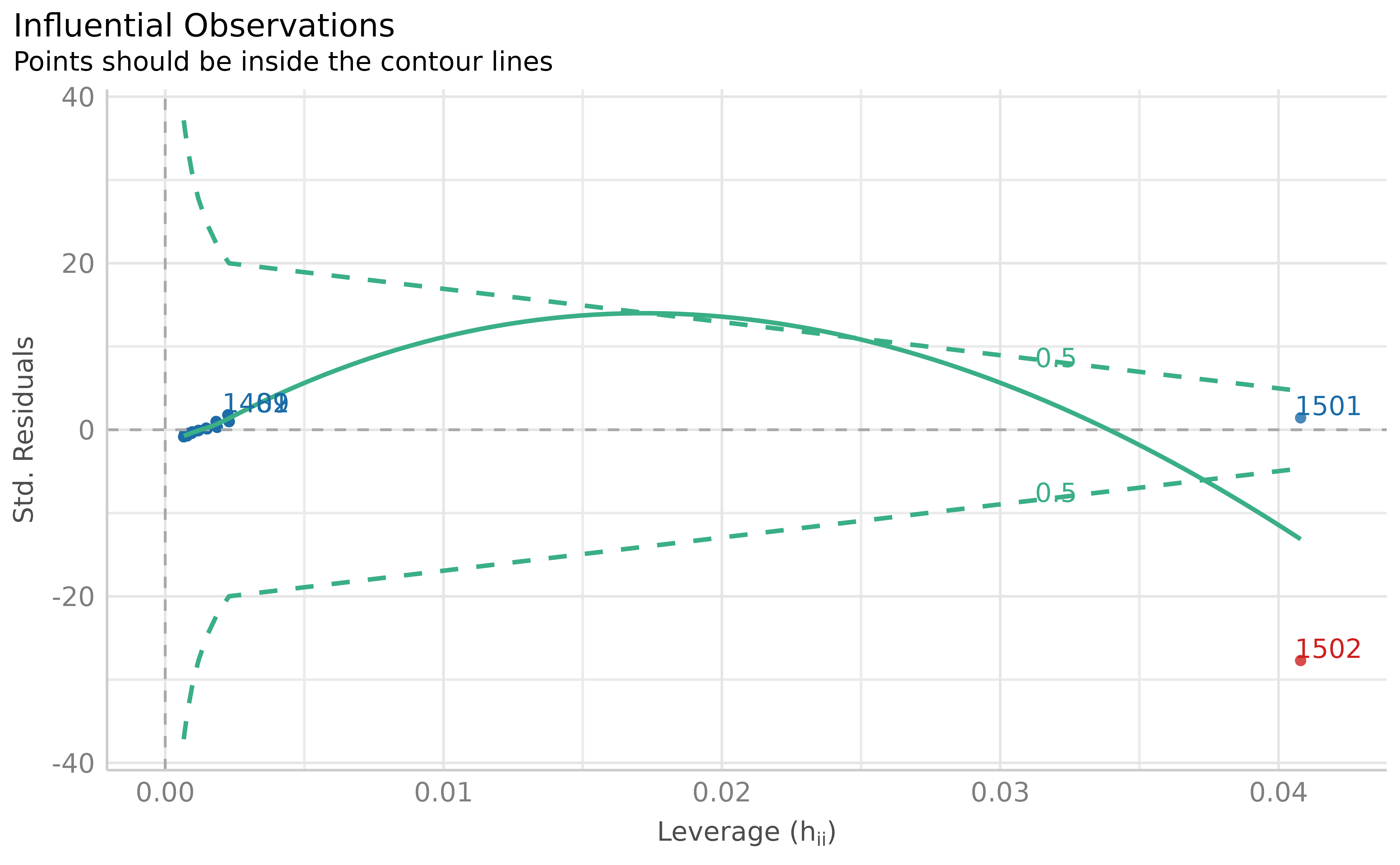
The leverage method (Cook’s distance) correctly distinguishes the true outlier from the model-consistent extreme observation), based on the fitted model.
Finally, unusual observations happen naturally: extreme observations are expected even when taken from a normal distribution. While statistical models can integrate this “expectation”, multivariate outlier methods might be too conservative, flagging too many observations despite belonging to the right generative process. For these reasons, we believe that model-based methods are still preferable to the MCD when using supported regression models. Additionally, if the presence of multiple outliers is a significant concern, regression methods that are more robust to outliers should be considered—like t regression or quantile regression—as they render their precise identification less critical (McElreath 2020).
Composite Outlier Score
The {performance} package also offers an alternative, consensus-based approach that combines several methods, based on the assumption that different methods provide different angles of looking at a given problem. By applying a variety of methods, one can hope to “triangulate” the true outliers (those consistently flagged by multiple methods) and thus attempt to minimize false positives.
In practice, this approach computes a composite outlier score, formed
of the average of the binary (0 or 1) classification results of each
method. It represents the probability that each observation is
classified as an outlier by at least one method. The default decision
rule classifies rows with composite outlier scores superior or equal to
0.5 as outlier observations (i.e., that were classified as outliers by
at least half of the methods). In {performance}’s
check_outliers(), one can use this approach by including
all desired methods in the corresponding argument.
outliers <- check_outliers(model, method = c("zscore_robust", "mcd", "cook"), verbose = FALSE)
which(outliers)
> [1] 1501 1502Outliers (counts or per variables) for individual methods can then be obtained through attributes. For example:
attributes(outliers)$outlier_var$zscore_robust> $weight
> Row Distance_Zscore_robust
> 1501 1501 6.9
> 1502 1502 3.7
>
> $height
> Row Distance_Zscore_robust
> 1501 1501 5.9
> 1502 1502 5.9An example sentence for reporting the usage of the composite method could be:
Based on a composite outlier score (see the ‘check_outliers()’ function in the ‘performance’ R package, Lüdecke et al. 2021) obtained via the joint application of multiple outliers detection algorithms ((a) median absolute deviation (MAD)-based robust z scores, Leys et al. 2013; (b) Mahalanobis minimum covariance determinant (MCD), Leys et al. 2019; and (c) Cook’s distance, Cook 1977), we excluded two participants that were classified as outliers by at least half of the methods used.
Handling Outliers
The above section demonstrated how to identify outliers using the
check_outliers() function in the {performance}
package. But what should we do with these outliers once identified?
Although it is common to automatically discard any observation that has
been marked as “an outlier” as if it might infect the rest of the data
with its statistical ailment, we believe that the use of SOD methods is
but one step in the get-to-know-your-data pipeline; a researcher or
analyst’s domain knowledge must be involved in the decision of
how to deal with observations marked as outliers by means of SOD.
Indeed, automatic tools can help detect outliers, but they are nowhere
near perfect. Although they can be useful to flag suspect data, they can
have misses and false alarms, and they cannot replace human eyes and
proper vigilance from the researcher. If you do end up manually
inspecting your data for outliers, it can be helpful to think of
outliers as belonging to different types of outliers, or categories,
which can help decide what to do with a given outlier.
Error, Interesting, and Random Outliers
Leys et al. (2019) distinguish between error outliers, interesting outliers, and random outliers. Error outliers are likely due to human error and should be corrected before data analysis or outright removed since they are invalid observations. Interesting outliers are not due to technical error and may be of theoretical interest; it might thus be relevant to investigate them further even though they should be removed from the current analysis of interest. Random outliers are assumed to be due to chance alone and to belong to the correct distribution and, therefore, should be retained.
It is recommended to keep observations which are expected to be part of the distribution of interest, even if they are outliers (Leys et al. 2019). However, if it is suspected that the outliers belong to an alternative distribution, then those observations could have a large impact on the results and call into question their robustness, especially if significance is conditional on their inclusion, so should be removed.
We should also keep in mind that there might be error outliers that are not detected by statistical tools, but should nonetheless be found and removed. For example, if we are studying the effects of X on Y among teenagers and we have one observation from a 20-year-old, this observation might not be a statistical outlier, but it is an outlier in the context of our research, and should be discarded. We could call these observations undetected error outliers, in the sense that although they do not statistically stand out, they do not belong to the theoretical or empirical distribution of interest (e.g., teenagers). In this way, we should not blindly rely on statistical outlier detection methods; doing our due diligence to investigate undetected error outliers relative to our specific research question is also essential for valid inferences.
Winsorization
Removing outliers can in this case be a valid strategy, and ideally one would report results with and without outliers to see the extent of their impact on results. This approach however can reduce statistical power. Therefore, some propose a recoding approach, namely, winsorization: bringing outliers back within acceptable limits (e.g., 3 MADs, Tukey and McLaughlin 1963). However, if possible, it is recommended to collect enough data so that even after removing outliers, there is still sufficient statistical power without having to resort to winsorization (Leys et al. 2019).
The easystats ecosystem makes it easy to incorporate this
step into your workflow through the winsorize() function of
{datawizard}, a lightweight R package to facilitate data
wrangling and statistical transformations (Patil
et al. 2022). This procedure will bring back univariate outliers
within the limits of ‘acceptable’ values, based either on the
percentile, the z score, or its robust alternative based on the
MAD.
data[1501:1502, ] # See outliers rows> height weight
> 1501 100 258
> 1502 100 200
# Winsorizing using the MAD
library(datawizard)
winsorized_data <- winsorize(data, method = "zscore", robust = TRUE, threshold = 3)
# Values > +/- MAD have been winsorized
winsorized_data[1501:1502, ]
> height weight
> 1501 83 188
> 1502 83 188The Importance of Transparency
Once again, it is a critical part of a sound outlier treatment that regardless of which SOD method used, it should be reported in a reproducible manner. Ideally, the handling of outliers should be specified a priori with as much detail as possible, and preregistered, to limit researchers’ degrees of freedom and therefore risks of false positives (Leys et al. 2019). This is especially true given that interesting outliers and random outliers are often times hard to distinguish in practice. Thus, researchers should always prioritize transparency and report all of the following information: (a) how many outliers were identified (including percentage); (b) according to which method and criteria, (c) using which function of which R package (if applicable), and (d) how they were handled (excluded or winsorized, if the latter, using what threshold). If at all possible, (e) the corresponding code script along with the data should be shared on a public repository like the Open Science Framework (OSF), so that the exclusion criteria can be reproduced precisely.
Conclusion
In this vignette, we have showed how to investigate outliers using
the check_outliers() function of the {performance}
package while following current good practices. However, best practice
for outlier treatment does not stop at using appropriate statistical
algorithms, but entails respecting existing recommendations, such as
preregistration, reproducibility, consistency, transparency, and
justification. Ideally, one would additionally also report the package,
function, and threshold used (linking to the full code when possible).
We hope that this paper and the accompanying
check_outlier() function of easystats will help
researchers engage in good research practices while providing a smooth
outlier detection experience.