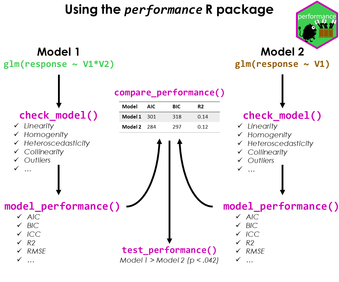
Analytic workflow: Assessing model fit • easystats

This vignette shows how to use the performance package to check the fit of a model, how to detect misspecification and how to improve your model. The basic workflow of the performance package can be summarized as follows:

fit a regression model
check the model fit and assess model fit indices
if necessary, fit another model that could potentially improve the fit
compare the model fit indices and perform statistical tests to determine which model is the best fit

In the following, we will demonstrate this workflow using a model with a count response variable. We will fit a Poisson regression model to the Salamanders dataset from the glmmTMB package. The dataset contains counts of salamanders in different sites, along with information on the number of mines and the species of salamanders. We will check the model fit and assess the model fit indices.

Problems that may arise with count response variables are zero inflation and overdispersion. Zero inflation occurs when there are more zeros in the data than expected under the Poisson distribution. Overdispersion occurs when the variance of the data is greater than the mean, which violates the assumption of equidispersion in the Poisson distribution.

We will check for these problems and suggest ways to improve the model fit, i.e. if necessary, we will fit another model that could potentially improve the fit. Finally, we will compare the model fit indices and perform statistical tests to determine which model is the best fit.

Fit the initial model

We start with a generalized mixed effects model, using a Poisson distribution.

library(performance)
model1 <- glmmTMB::glmmTMB(
  count ~ mined + spp + (1 | site),
  family = poisson,
  data = glmmTMB::Salamanders
)

First, let us look at the summary of the model.

library(parameters)
model_parameters(model1)
#> # Fixed Effects
#> 
#> Parameter   | Log-Mean |   SE |         95% CI |     z |      p
#> ---------------------------------------------------------------
#> (Intercept) |    -1.62 | 0.24 | [-2.10, -1.15] | -6.76 | < .001
#> mined [no]  |     2.26 | 0.28 | [ 1.72,  2.81] |  8.08 | < .001
#> spp [PR]    |    -1.39 | 0.22 | [-1.81, -0.96] | -6.44 | < .001
#> spp [DM]    |     0.23 | 0.13 | [-0.02,  0.48] |  1.79 | 0.074 
#> spp [EC-A]  |    -0.77 | 0.17 | [-1.11, -0.43] | -4.50 | < .001
#> spp [EC-L]  |     0.62 | 0.12 | [ 0.39,  0.86] |  5.21 | < .001
#> spp [DES-L] |     0.68 | 0.12 | [ 0.45,  0.91] |  5.75 | < .001
#> spp [DF]    |     0.08 | 0.13 | [-0.18,  0.34] |  0.60 | 0.549 
#> 
#> # Random Effects
#> 
#> Parameter            | Coefficient |       95% CI
#> -------------------------------------------------
#> SD (Intercept: site) |        0.58 | [0.38, 0.87]
#> 
#> Uncertainty intervals (equal-tailed) and p-values (two-tailed) computed
#>   using a Wald z-distribution approximation.
#> 
#> The model has a log- or logit-link. Consider using `exponentiate =
#>   TRUE` to interpret coefficients as ratios.

We see a lot of statistically significant estimates here. No matter, which philosophy you follow in terms of interpreting statistical test results, our conclusions we draw from our regression models will be inaccurate if our modeling assumptions are a poor fit for the situation. Hence, checking model fit is essential.

In performance, we can conduct a comprehensive visual inspection of our model fit using check_model(). We won’t go into details of all the plots here, but you can find more information on all created diagnostic plots in the dedicated vignette.

For now, we want to focus on the posterior predictive checks, dispersion and zero-inflation as well as the Q-Q plot (uniformity of residuals).

check_model(model1)
#> `check_outliers()` does not yet support models of class `glmmTMB`.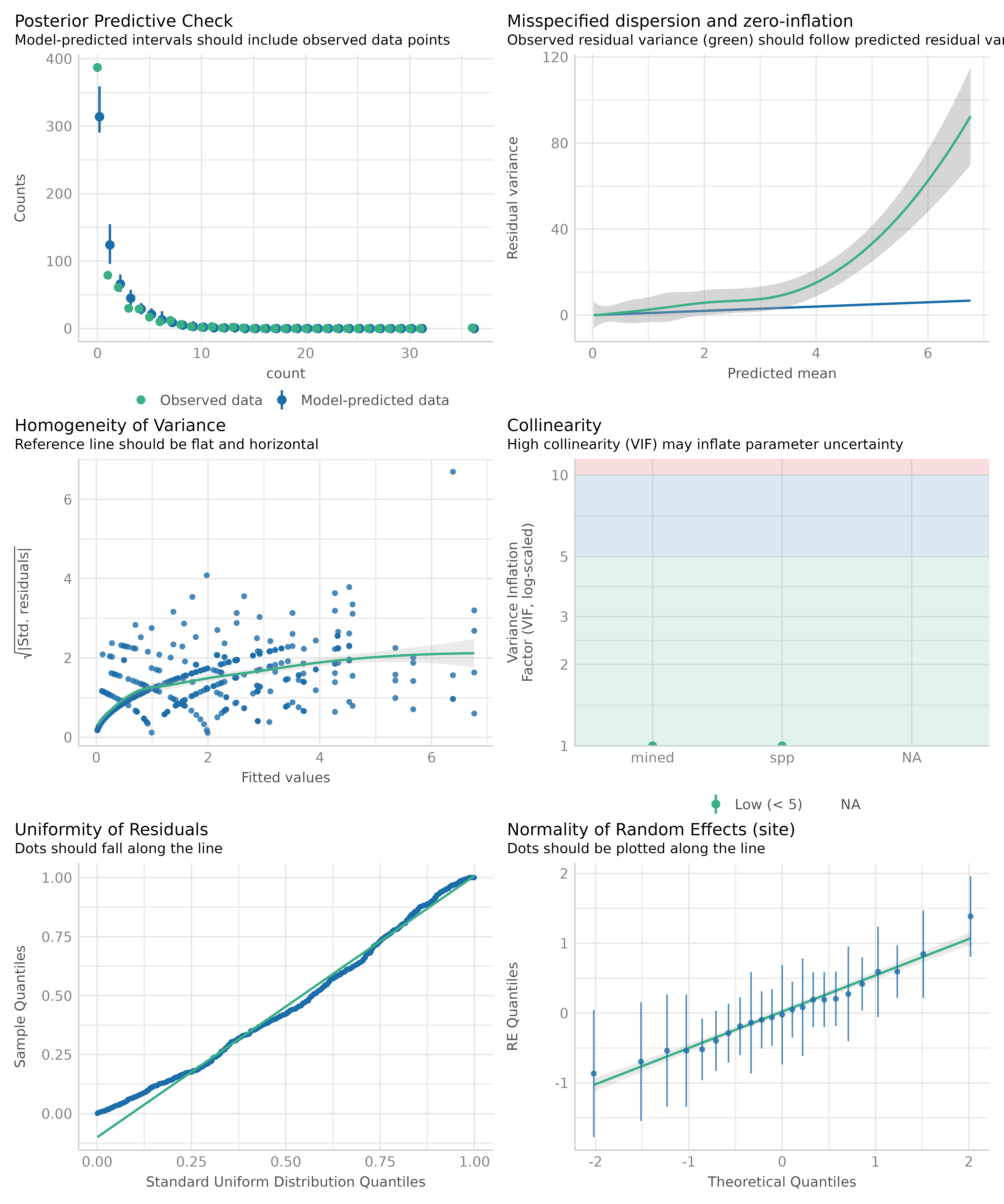

Note that unlike plot(), which is a base R function to create diagnostic plots, check_model() relies on simulated residuals for the Q-Q plot, which is more accurate for non-Gaussian models. See this vignette and the documentation of simulate_residuals() for further details.

The above plot suggests that we may have issues with overdispersion and/or zero-inflation. We can check for these problems using check_overdispersion() and check_zeroinflation(), which will perform statistical tests (based on simulated residuals). These tests can additionally be used beyond the visual inspection.

check_overdispersion(model1)
#> # Overdispersion test
#> 
#>        dispersion ratio =    2.324
#>   Pearson's Chi-Squared = 1475.875
#>                 p-value =  < 0.001
#> Overdispersion detected.

check_zeroinflation(model1)
#> # Check for zero-inflation
#> 
#>    Observed zeros: 387
#>   Predicted zeros: 311
#>             Ratio: 0.80
#> Model is underfitting zeros (probable zero-inflation).

As we can see, our model seems to suffer both from overdispersion and zero-inflation.

First attempt at improving the model fit

We can try to improve the model fit by fitting a model with zero-inflation component:

model2 <- glmmTMB::glmmTMB(
  count ~ mined + spp + (1 | site),
  ziformula = ~ mined + spp,
  family = poisson,
  data = glmmTMB::Salamanders
)
check_model(model2)
#> `check_outliers()` does not yet support models of class `glmmTMB`.

Looking at the above plots, the zero-inflation seems to be addressed properly (see especially posterior predictive checks and uniformity of residuals, the Q-Q plot). However, the overdispersion still could be present. We can check for these problems using check_overdispersion() and check_zeroinflation() again.

check_overdispersion(model2)
#> # Overdispersion test
#> 
#>  dispersion ratio = 1.679
#>           p-value = 0.008
#> Overdispersion detected.

check_zeroinflation(model2)
#> # Check for zero-inflation
#> 
#>    Observed zeros: 387
#>   Predicted zeros: 387
#>             Ratio: 1.00
#> Model seems ok, ratio of observed and predicted zeros is within the
#>   tolerance range (p > .999).

Indeed, the overdispersion is still present.

Second attempt at improving the model fit

We can try to address this issue by fitting a negative binomial model instead of using a Poisson distribution.

model3 <- glmmTMB::glmmTMB(
  count ~ mined + spp + (1 | site),
  ziformula = ~ mined + spp,
  family = glmmTMB::nbinom1,
  data = glmmTMB::Salamanders
)
check_model(model3)
#> `check_outliers()` does not yet support models of class `glmmTMB`.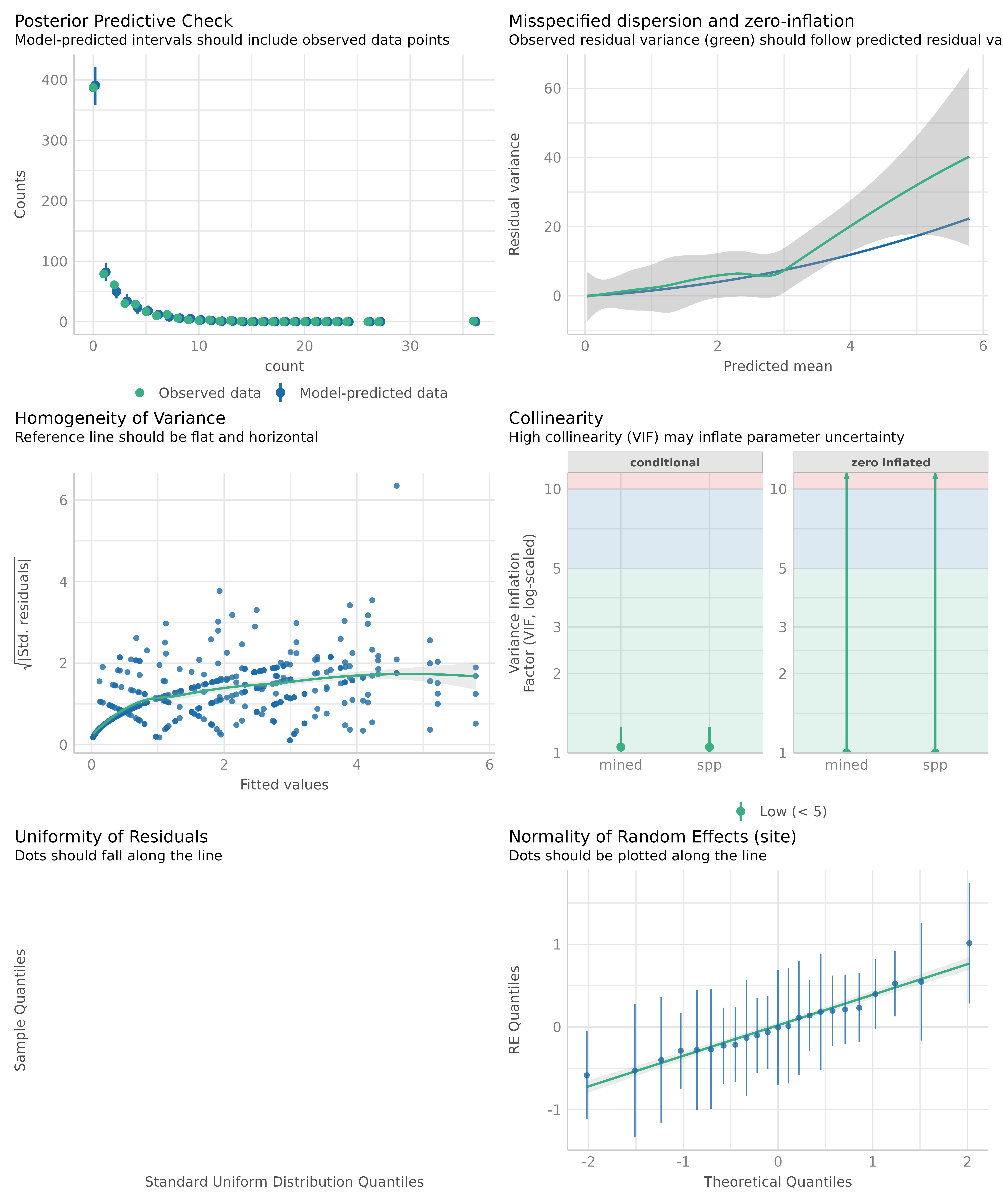

Now we see that the plot showing misspecified dispersion and zero-inflation suggests that the overdispersion is better addressed than before. Let us check again:

check_overdispersion(model3)
#> # Overdispersion test
#> 
#>  dispersion ratio = 1.081
#>           p-value =  0.54
#> No overdispersion detected.

check_zeroinflation(model3)
#> # Check for zero-inflation
#> 
#>    Observed zeros: 387
#>   Predicted zeros: 389
#>             Ratio: 1.00
#> Model seems ok, ratio of observed and predicted zeros is within the
#>   tolerance range (p > .999).

Comparing model fit indices

There are different model fit indices that can be used to compare models. For our purpose, we rely on the Akaike Information Criterion (AIC), the corrected Akaike Information Criterion (AICc), the Bayesian Information Criterion (BIC), and the Proper Scoring Rules. We can compare the models using compare_performance() and plot().

result <- compare_performance(
  model1, model2, model3,
  metrics = c("AIC", "AICc", "BIC", "SCORE")
)
result
#> # Comparison of Model Performance Indices
#> 
#> Name   |   Model |  AIC (weights) | AICc (weights) |  BIC (weights) | Score_log | Score_spherical
#> -------------------------------------------------------------------------------------------------
#> model1 | glmmTMB | 1962.8 (<.001) | 1963.1 (<.001) | 2003.0 (<.001) |    -1.457 |           0.032
#> model2 | glmmTMB | 1785.5 (<.001) | 1786.5 (<.001) | 1861.4 (<.001) |    -1.328 |           0.032
#> model3 | glmmTMB | 1653.7 (>.999) | 1654.8 (>.999) | 1734.1 (>.999) |    -1.275 |           0.032

plot(result)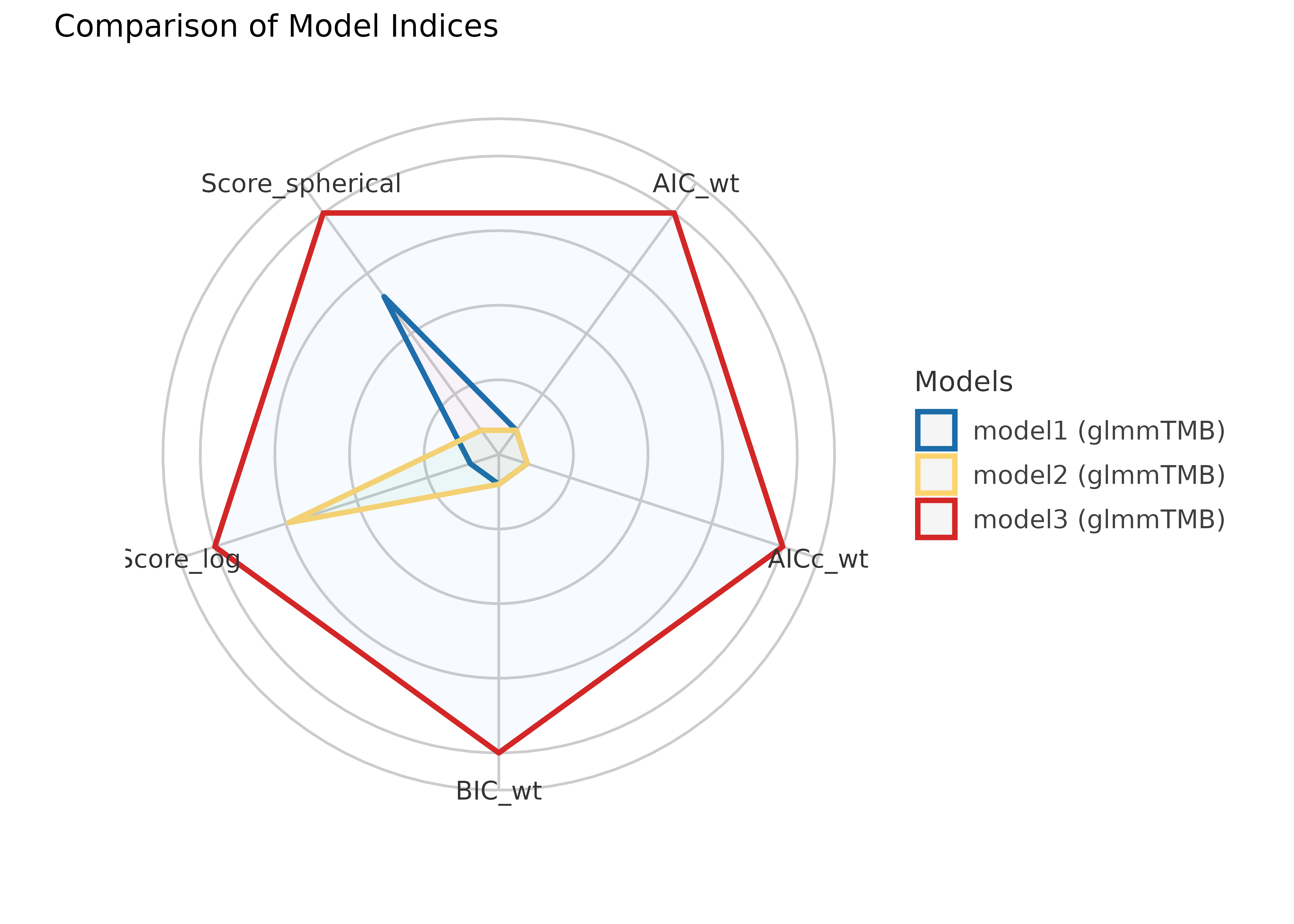

The weighted AIC and BIC range from 0 to 1, indicating better model fit the closer the value is to 1. The AICc is a corrected version of the AIC for small sample sizes. The Proper Scoring Rules range from -Inf to 0, with higher values (i.e. closer to 0) indicating better model fit.

The above results suggest that indeed our third model is the best fit.

Statistical tests for model comparison

We can also perform statistical tests to determine which model is the best fit using test_performance() or anova(). test_performance() automatically selects an appropriate test based on the model family. You can also call the different tests, like test_likelihoodratio(), test_bf(), test_wald() or test_vuong() directly.

test_performance(model1, model2, model3)
#> Name   |   Model |     BF | df | df_diff |   Chi2 |      p
#> ----------------------------------------------------------
#> model1 | glmmTMB |        |  9 |         |        |       
#> model2 | glmmTMB | > 1000 | 17 |    8.00 | 193.31 | < .001
#> model3 | glmmTMB | > 1000 | 18 |    1.00 | 133.83 | < .001
#> Models were detected as nested (in terms of fixed parameters) and are compared in sequential order.

We see, first, that test_performance() used the Bayes factor (based on BIC comparison) to compare the models. And second, that both the second and third model seem to be significantly better than the first model.

Now we compare the second against the third model

test_performance(model2, model3)
#> Name   |   Model |     BF | df | df_diff |   Chi2 |      p
#> ----------------------------------------------------------
#> model2 | glmmTMB |        | 17 |         |        |       
#> model3 | glmmTMB | > 1000 | 18 |    1.00 | 133.83 | < .001
#> Models were detected as nested (in terms of fixed parameters) and are compared in sequential order.

test_likelihoodratio(model2, model3)
#> # Likelihood-Ratio-Test (LRT) for Model Comparison (ML-estimator)
#> 
#> Name   |   Model | df | df_diff |   Chi2 |      p
#> -------------------------------------------------
#> model2 | glmmTMB | 17 |         |        |       
#> model3 | glmmTMB | 18 |       1 | 133.83 | < .001

We see that both the Bayes factor and likelihood ratio test suggest that the third model is significantly better than the second model.

What does this mean for our inference?

model_parameters(model3)
#> # Fixed Effects (Count Model)
#> 
#> Parameter   | Log-Mean |   SE |         95% CI |     z |      p
#> ---------------------------------------------------------------
#> (Intercept) |    -0.75 | 0.34 | [-1.40, -0.09] | -2.23 | 0.026 
#> mined [no]  |     1.56 | 0.33 | [ 0.92,  2.20] |  4.78 | < .001
#> spp [PR]    |    -1.57 | 0.30 | [-2.16, -0.97] | -5.15 | < .001
#> spp [DM]    |     0.07 | 0.20 | [-0.32,  0.46] |  0.34 | 0.735 
#> spp [EC-A]  |    -0.93 | 0.27 | [-1.45, -0.41] | -3.51 | < .001
#> spp [EC-L]  |     0.31 | 0.20 | [-0.07,  0.69] |  1.59 | 0.111 
#> spp [DES-L] |     0.41 | 0.19 | [ 0.04,  0.79] |  2.19 | 0.028 
#> spp [DF]    |    -0.12 | 0.20 | [-0.51,  0.28] | -0.57 | 0.568 
#> 
#> # Fixed Effects (Zero-Inflation Component)
#> 
#> Parameter   | Log-Odds |       SE |                 95% CI |         z |      p
#> -------------------------------------------------------------------------------
#> (Intercept) |     2.28 |     1.12 | [      0.08,     4.47] |      2.04 | 0.042 
#> mined [no]  |   -21.36 |  4655.41 | [  -9145.81,  9103.08] | -4.59e-03 | 0.996 
#> spp [PR]    |   -24.37 | 92198.78 | [ -1.81e+05, 1.81e+05] | -2.64e-04 | > .999
#> spp [DM]    |    -3.63 |     2.01 | [     -7.57,     0.31] |     -1.80 | 0.071 
#> spp [EC-A]  |    -2.79 |     1.95 | [     -6.61,     1.03] |     -1.43 | 0.152 
#> spp [EC-L]  |    -2.84 |     1.41 | [     -5.59,    -0.08] |     -2.02 | 0.044 
#> spp [DES-L] |    -3.56 |     1.78 | [     -7.04,    -0.07] |     -2.00 | 0.045 
#> spp [DF]    |   -20.55 |  4284.59 | [  -8418.20,  8377.09] | -4.80e-03 | 0.996 
#> 
#> # Dispersion
#> 
#> Parameter   | Coefficient |       95% CI
#> ----------------------------------------
#> (Intercept) |        2.02 | [1.54, 2.67]
#> 
#> # Random Effects Variances
#> 
#> Parameter            | Coefficient |       95% CI
#> -------------------------------------------------
#> SD (Intercept: site) |        0.46 | [0.27, 0.76]
#> 
#> Uncertainty intervals (equal-tailed) and p-values (two-tailed) computed
#>   using a Wald z-distribution approximation.

Obviously, although we might have found the best fitting model, coefficients for the zero-inflation component of our model look rather spurious. We have very high coefficients here. We still might find a better distributional family for our model, and try nbinom2 now.

model4 <- glmmTMB::glmmTMB(
  count ~ mined + spp + (1 | site),
  ziformula = ~ mined + spp,
  family = glmmTMB::nbinom2,
  data = glmmTMB::Salamanders
)
check_model(model4)
#> `check_outliers()` does not yet support models of class `glmmTMB`.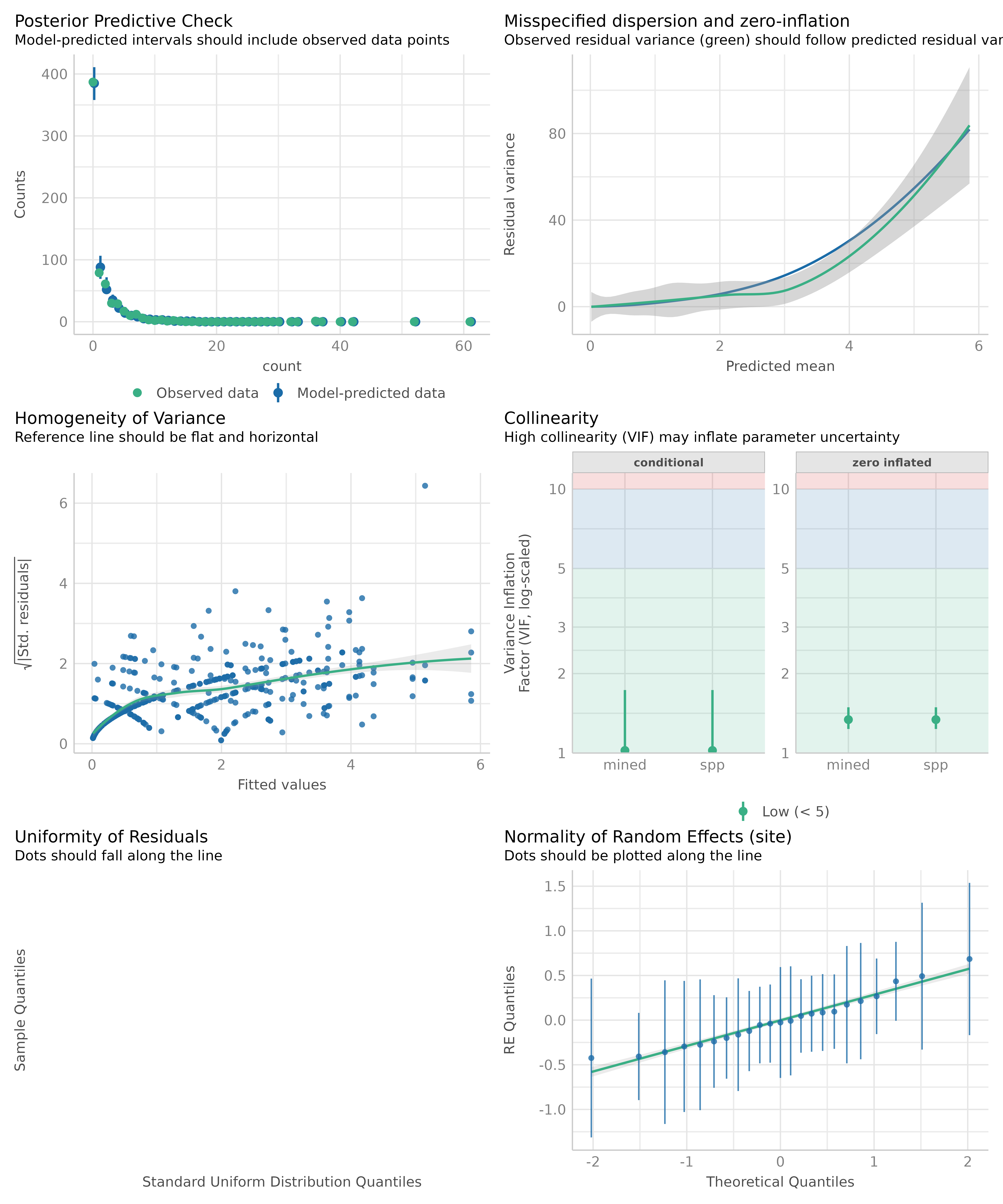


check_overdispersion(model4)
#> # Overdispersion test
#> 
#>  dispersion ratio = 0.958
#>           p-value =  0.93
#> No overdispersion detected.

check_zeroinflation(model4)
#> # Check for zero-inflation
#> 
#>    Observed zeros: 387
#>   Predicted zeros: 386
#>             Ratio: 1.00
#> Model seems ok, ratio of observed and predicted zeros is within the
#>   tolerance range (p = 0.952).

test_likelihoodratio(model3, model4)
#> Some of the nested models seem to be identical and probably only vary in
#>   their random effects.
#> # Likelihood-Ratio-Test (LRT) for Model Comparison (ML-estimator)
#> 
#> Name   |   Model | df | df_diff |  Chi2 |      p
#> ------------------------------------------------
#> model3 | glmmTMB | 18 |         |       |       
#> model4 | glmmTMB | 18 |       0 | 16.64 | < .001

model_parameters(model4)
#> # Fixed Effects (Count Model)
#> 
#> Parameter   | Log-Mean |   SE |        95% CI |     z |      p
#> --------------------------------------------------------------
#> (Intercept) |    -0.61 | 0.41 | [-1.40, 0.18] | -1.51 | 0.132 
#> mined [no]  |     1.43 | 0.37 | [ 0.71, 2.15] |  3.90 | < .001
#> spp [PR]    |    -0.96 | 0.64 | [-2.23, 0.30] | -1.50 | 0.134 
#> spp [DM]    |     0.17 | 0.24 | [-0.29, 0.63] |  0.73 | 0.468 
#> spp [EC-A]  |    -0.39 | 0.34 | [-1.06, 0.28] | -1.13 | 0.258 
#> spp [EC-L]  |     0.49 | 0.24 | [ 0.02, 0.96] |  2.05 | 0.041 
#> spp [DES-L] |     0.59 | 0.23 | [ 0.14, 1.04] |  2.59 | 0.010 
#> spp [DF]    |    -0.11 | 0.24 | [-0.59, 0.36] | -0.46 | 0.642 
#> 
#> # Fixed Effects (Zero-Inflation Component)
#> 
#> Parameter   | Log-Odds |   SE |         95% CI |     z |      p
#> ---------------------------------------------------------------
#> (Intercept) |     0.91 | 0.63 | [-0.32,  2.14] |  1.45 | 0.147 
#> mined [no]  |    -2.56 | 0.60 | [-3.75, -1.38] | -4.24 | < .001
#> spp [PR]    |     1.16 | 1.33 | [-1.45,  3.78] |  0.87 | 0.384 
#> spp [DM]    |    -0.94 | 0.80 | [-2.51,  0.63] | -1.17 | 0.241 
#> spp [EC-A]  |     1.04 | 0.71 | [-0.36,  2.44] |  1.46 | 0.144 
#> spp [EC-L]  |    -0.56 | 0.73 | [-1.99,  0.86] | -0.77 | 0.439 
#> spp [DES-L] |    -0.89 | 0.75 | [-2.37,  0.58] | -1.19 | 0.236 
#> spp [DF]    |    -2.54 | 2.18 | [-6.82,  1.74] | -1.16 | 0.244 
#> 
#> # Dispersion
#> 
#> Parameter   | Coefficient |       95% CI
#> ----------------------------------------
#> (Intercept) |        1.51 | [0.93, 2.46]
#> 
#> # Random Effects Variances
#> 
#> Parameter            | Coefficient |       95% CI
#> -------------------------------------------------
#> SD (Intercept: site) |        0.38 | [0.17, 0.87]
#> 
#> Uncertainty intervals (equal-tailed) and p-values (two-tailed) computed
#>   using a Wald z-distribution approximation.

Based on these results, we might even go with model4.

Conclusion

Statistics is hard. It is not just about fitting a model, but also about checking the model fit and improving the model. This also requires domain knowledge to consider whether all relevant predictors are included in the model (and whether all included predictors are relevant!).

The performance package provides a comprehensive set of tools to help you with this task. We have demonstrated how to use these tools to check the fit of a model, detect misspecification, and improve the model. We have also shown how to compare the model fit indices and perform statistical tests to determine which model is the best fit. We hope this vignette has been helpful in guiding you through this process.