This vignette can be cited as:
citation("correlation")> To cite package 'correlation' in publications use:
>
> Makowski, D., Wiernik, B. M., Patil, I., Lüdecke, D., & Ben-Shachar,
> M. S. (2022). correlation: Methods for correlation analysis (0.8.3)
> [R package]. https://CRAN.R-project.org/package=correlation (Original
> work published 2020)
>
> Makowski, D., Ben-Shachar, M. S., Patil, I., & Lüdecke, D. (2019).
> Methods and algorithms for correlation analysis in R. Journal of Open
> Source Software, 5(51), 2306. https://doi.org/10.21105/joss.02306
>
> To see these entries in BibTeX format, use 'print(<citation>,
> bibtex=TRUE)', 'toBibtex(.)', or set
> 'options(citation.bibtex.max=999)'.Different Methods for Correlations
Correlations tests are arguably one of the most commonly used statistical procedures, and are used as a basis in many applications such as exploratory data analysis, structural modeling, data engineering, etc. In this context, we present correlation, a toolbox for the R language (R Core Team 2019) and part of the easystats collection, focused on correlation analysis. Its goal is to be lightweight, easy to use, and allows for the computation of many different kinds of correlations, such as:
- Pearson’s correlation: This is the most common correlation method. It corresponds to the covariance of the two variables normalized (i.e., divided) by the product of their standard deviations.
r_{xy} = \frac{cov(x,y)}{SD_x \times SD_y}
- Spearman’s rank correlation: A non-parametric measure of correlation, the Spearman correlation between two variables is equal to the Pearson correlation between the rank scores of those two variables; while Pearson’s correlation assesses linear relationships, Spearman’s correlation assesses monotonic relationships (whether linear or not). Confidence Intervals (CI) for Spearman’s correlations are computed using the Fieller et al. (1957) correction (see Bishara and Hittner 2017).
r_{s_{xy}} = \frac{cov(rank_x, rank_y)}{SD(rank_x) \times SD(rank_y)}
- Kendall’s rank correlation: In the normal case, the Kendall correlation is preferred to the Spearman correlation because of a smaller gross error sensitivity (GES) and a smaller asymptotic variance (AV), making it more robust and more efficient. However, the interpretation of Kendall’s tau is less direct compared to that of the Spearman’s rho, in the sense that it quantifies the difference between the % of concordant and discordant pairs among all possible pairwise events. Confidence Intervals (CI) for Kendall’s correlations are computed using the Fieller et al. (1957) correction (see Bishara and Hittner 2017). For each pair of observations (i ,j) of two variables (x, y), it is defined as follows:
\tau_{xy} = \frac{2}{n(n-1)}\sum_{i<j}^{}sign(x_i - x_j) \times sign(y_i - y_j)
Biweight midcorrelation: A measure of similarity that is median-based, instead of the traditional mean-based, thus being less sensitive to outliers. It can be used as a robust alternative to other similarity metrics, such as Pearson correlation (Langfelder and Horvath 2012).
Distance correlation: Distance correlation measures both linear and non-linear association between two random variables or random vectors (for more, see Székely et al. (2007), Székely and Rizzo (2009)). This is in contrast to Pearson’s correlation, which can only detect linear association between two random variables.
Percentage bend correlation: Introduced by Wilcox (1994), it is based on a down-weight of a specified percentage of marginal observations deviating from the median (by default, 20 percent).
Shepherd’s Pi correlation: Equivalent to a Spearman’s rank correlation after outliers removal (by means of bootstrapped Mahalanobis distance).
Blomqvist’s coefficient: The Blomqvist’s coefficient (also referred to as Blomqvist’s Beta or medial correlation; Blomqvist, 1950) is a median-based non-parametric correlation that has some advantages over measures such as Spearman’s or Kendall’s estimates (see Shmid and Schimdt, 2006).
Hoeffding’s D: The Hoeffding’s D statistic is a non-parametric rank based measure of association that detects more general departures from independence (Hoeffding 1948), including non-linear associations. Hoeffding’s D varies between -0.5 and 1 (if there are no tied ranks, otherwise it can have lower values), with larger values indicating a stronger relationship between the variables.
Gamma correlation: The Goodman-Kruskal gamma statistic is similar to Kendall’s Tau coefficient. It is relatively robust to outliers and deals well with data that have many ties.
Gaussian rank correlation: The Gaussian rank correlation estimator is a simple and well-performing alternative for robust rank correlations (Boudt et al., 2012). It is based on the Gaussian quantiles of the ranks.
Point-Biserial and biserial correlation: Correlation coefficient used when one variable is continuous and the other is dichotomous (binary). Point-Biserial is equivalent to a Pearson’s correlation, while Biserial should be used when the binary variable is assumed to have an underlying continuity. For example, anxiety level can be measured on a continuous scale, but can be classified dichotomously as high/low.
Winsorized correlation: Correlation of variables that have been Winsorized, i.e., transformed by limiting extreme values to reduce the effect of possibly spurious outliers.
Polychoric correlation: Correlation between two theorised normally distributed continuous latent variables, from two observed ordinal variables.
Tetrachoric correlation: Special case of the polychoric correlation applicable when both observed variables are dichotomous.
Partial correlation: Correlation between two variables after adjusting for the (linear) effect of one or more variables. The correlation test is run after having partialized the dataset, independently from it. In other words, it considers partialization as an independent step generating a different dataset, rather than belonging to the same model. This is why some discrepancies are to be expected for the t- and the p-values (but not the correlation coefficient) compared to other implementations such as
ppcor. Let e_{x.z} be the residuals from the linear prediction of x by z (note that this can be expanded to a multivariate z):
r_{xy.z} = r_{e_{x.z},e_{y.z}}
- Multilevel correlation: Multilevel correlations are a special case of partial correlations where the variable to be adjusted for is a factor and is included as a random effect in a mixed-effects model.
Comparison
We will fit different types of correlations of generated data with different link strengths and link types.
Let’s first load the required libraries for this analysis.
library(correlation)
library(bayestestR)
library(see)
library(ggplot2)
library(datawizard)
library(poorman)
Utility functions
generate_results <- function(r, n = 100, transformation = "none") {
  data <- bayestestR::simulate_correlation(round(n), r = r)

  if (transformation != "none") {
    var <- ifelse(grepl("(", transformation, fixed = TRUE), "data$V2)", "data$V2")
    transformation <- paste0(transformation, var)
    data$V2 <- eval(parse(text = transformation))
  }

  out <- data.frame(n = n, transformation = transformation, r = r)

  out$Pearson <- cor_test(data, "V1", "V2", method = "pearson")$r
  out$Spearman <- cor_test(data, "V1", "V2", method = "spearman")$rho
  out$Kendall <- cor_test(data, "V1", "V2", method = "kendall")$tau
  out$Biweight <- cor_test(data, "V1", "V2", method = "biweight")$r
  out$Distance <- cor_test(data, "V1", "V2", method = "distance")$r
  out$Distance <- cor_test(data, "V1", "V2", method = "distance")$r

  out
}
Effect of Relationship Type
data <- data.frame()
for (r in seq(0, 0.999, length.out = 200)) {
  for (n in 100) {
    for (transformation in c(
      "none",
      "exp(",
      "log10(1+max(abs(data$V2))+",
      "1/",
      "tan(",
      "sin(",
      "cos(",
      "cos(2*",
      "abs(",
      "data$V2*",
      "data$V2*data$V2*",
      "ifelse(data$V2>0, 1, 0)*("
    )) {
      data <- rbind(data, generate_results(r, n, transformation = transformation))
    }
  }
}

data %>%
  datawizard::reshape_longer(
    select = -c("n", "r", "transformation"),
    names_to = "Type",
    values_to = "Estimation"
  ) %>%
  mutate(Type = relevel(as.factor(Type), "Pearson", "Spearman", "Kendall", "Biweight", "Distance")) %>%
  ggplot(aes(x = r, y = Estimation, fill = Type)) +
  geom_smooth(aes(color = Type), method = "loess", alpha = 0, na.rm = TRUE) +
  geom_vline(aes(xintercept = 0.5), linetype = "dashed") +
  geom_hline(aes(yintercept = 0.5), linetype = "dashed") +
  guides(colour = guide_legend(override.aes = list(alpha = 1))) +
  see::theme_modern() +
  scale_color_flat_d(palette = "rainbow") +
  scale_fill_flat_d(palette = "rainbow") +
  guides(colour = guide_legend(override.aes = list(alpha = 1))) +
  facet_wrap(~transformation)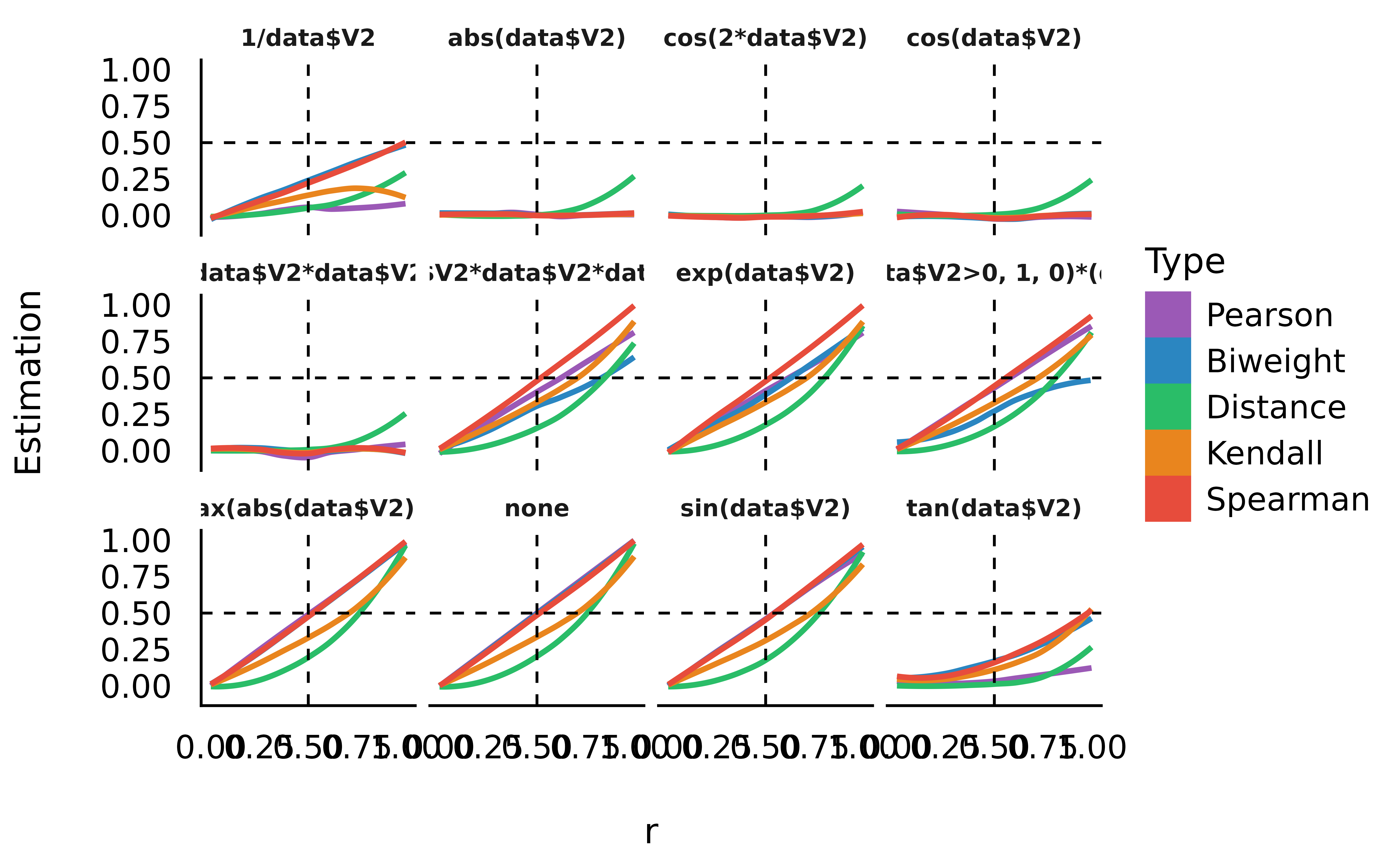
model <- data %>%
  datawizard::reshape_longer(
    select = -c("n", "r", "transformation"),
    names_to = "Type",
    values_to = "Estimation"
  ) %>%
  lm(r ~ Type / Estimation, data = .) %>%
  parameters::parameters()

arrange(model[6:10, ], desc(Coefficient))
> Parameter | Coefficient | SE | 95% CI | t(11903) | p
> ------------------------------------------------------------------------------------
> Type [Distance] × Estimation | 0.90 | 0.02 | [0.86, 0.95] | 40.14 | < .001
> Type [Kendall] × Estimation | 0.66 | 0.02 | [0.62, 0.70] | 32.07 | < .001
> Type [Biweight] × Estimation | 0.53 | 0.02 | [0.50, 0.57] | 29.24 | < .001
> Type [Spearman] × Estimation | 0.51 | 0.02 | [0.48, 0.54] | 31.70 | < .001
> Type [Pearson] × Estimation | 0.44 | 0.02 | [0.41, 0.47] | 26.49 | < .001As we can see, distance correlation is able to capture the strength even for severely non-linear relationships.