The plot() method for the bayestestR::rope().
Usage
# S3 method for class 'see_rope'
plot(
  x,
  data = NULL,
  alpha_rope = 0.5,
  color_rope = "cadetblue",
  show_intercept = FALSE,
  n_columns = 1,
  ...
)
Arguments
- x
An object.
- data
The original data used to create this object. Can be a statistical model.
- alpha_rope
Numeric specifying transparency level of ROPE ribbon.
- color_rope
Character specifying color of ROPE ribbon.
- show_intercept
Logical, if
TRUE, the intercept-parameter is included in the plot. By default, it is hidden because in many cases the intercept-parameter has a posterior distribution on a very different location, so density curves of posterior distributions for other parameters are hardly visible.- n_columns
For models with multiple components (like fixed and random, count and zero-inflated), defines the number of columns for the panel-layout. If
NULL, a single, integrated plot is shown.- ...
Arguments passed to or from other methods.
Examples
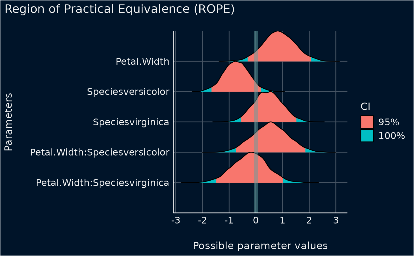
library(rstanarm)
library(bayestestR)
set.seed(123)
m <<- suppressWarnings(stan_glm(Sepal.Length ~ Petal.Width * Species, data = iris, refresh = 0))
result <- rope(m)
#> Possible multicollinearity between Petal.Width:Speciesversicolor and
#>   Petal.Width (r = 0.87), Petal.Width:Speciesvirginica and
#>   Petal.Width:Speciesversicolor (r = 0.79). This might lead to
#>   inappropriate results. See 'Details' in '?rope'.
result
#> # Proportion of samples inside the ROPE [-0.08, 0.08]:
#>
#> Parameter                     | Inside ROPE
#> -------------------------------------------
#> (Intercept)                   |      0.00 %
#> Petal.Width                   |      3.89 %
#> Speciesversicolor             |      4.63 %
#> Speciesvirginica              |      8.50 %
#> Petal.Width:Speciesversicolor |      6.79 %
#> Petal.Width:Speciesvirginica  |     10.74 %
#>
plot(result)