Plot method for simulated model parameters

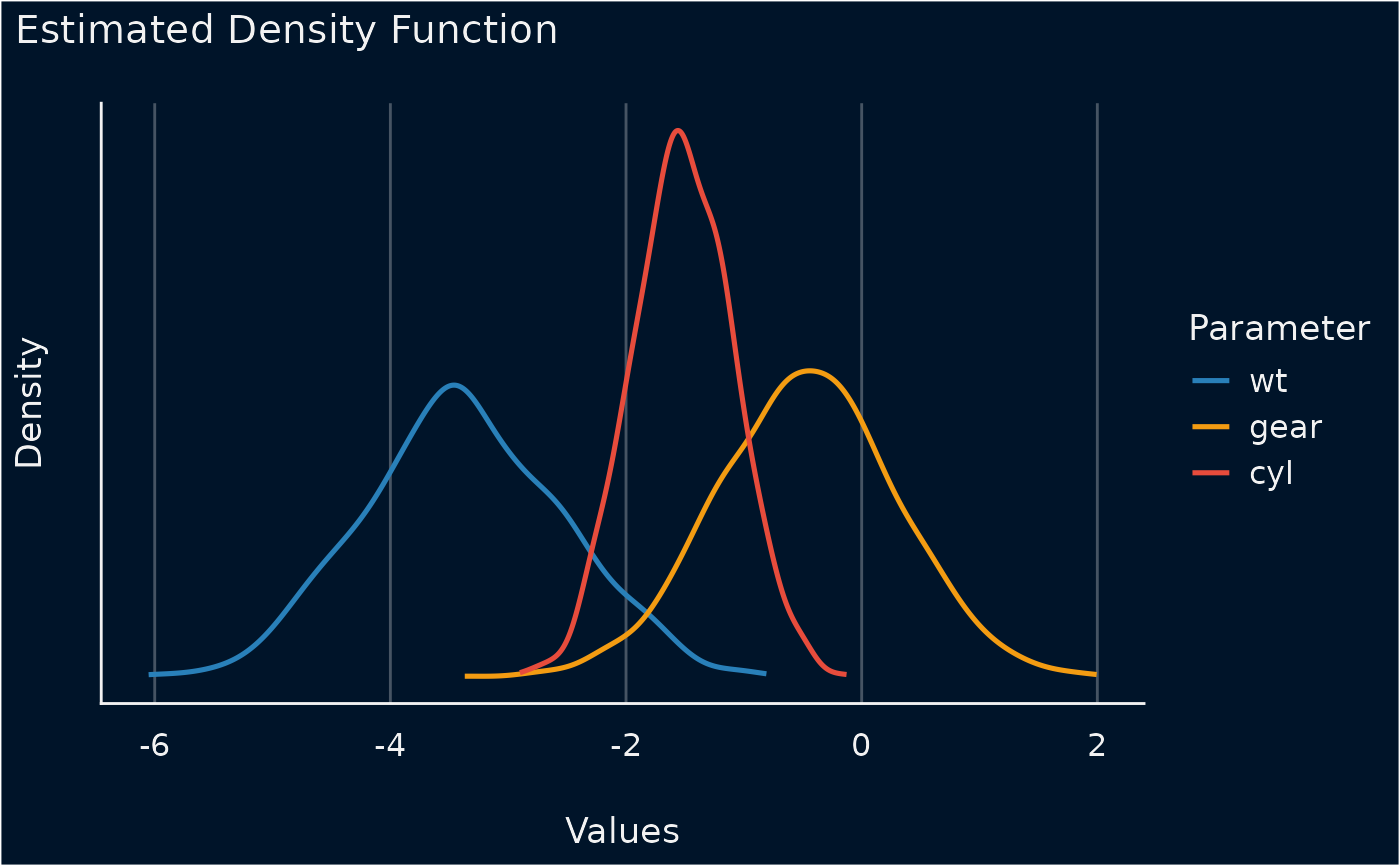
The plot() method for the parameters::simulate_parameters() function.

Usage

# S3 method for class 'see_parameters_simulate'
plot(
  x,
  data = NULL,
  stack = TRUE,
  show_intercept = FALSE,
  n_columns = NULL,
  normalize_height = FALSE,
  size_line = 0.9,
  posteriors_alpha = 0.7,
  centrality = "median",
  ci = 0.95,
  ...
)

Arguments

x

An object.

data

The original data used to create this object. Can be a statistical model.

stack

Logical. If TRUE, densities are plotted as stacked lines. Else, densities are plotted for each parameter among each other.

show_intercept

Logical, if TRUE, the intercept-parameter is included in the plot. By default, it is hidden because in many cases the intercept-parameter has a posterior distribution on a very different location, so density curves of posterior distributions for other parameters are hardly visible.

n_columns

For models with multiple components (like fixed and random, count and zero-inflated), defines the number of columns for the panel-layout. If NULL, a single, integrated plot is shown.

normalize_height

Logical. If TRUE, height of density-areas is "normalized", to avoid overlap. In certain cases when the range of a distribution of simulated draws is narrow for some parameters, this may result in very flat density-areas. In such cases, set normalize_height = FALSE.

size_line

Numeric value specifying size of line geoms.

posteriors_alpha

Numeric value specifying alpha for the posterior distributions.

centrality

Character specifying the point-estimate (centrality index) to compute. Can be "median", "mean" or "MAP".

ci

Numeric value of probability of the CI (between 0 and 1) to be estimated. Default to 0.95.

...

Arguments passed to or from other methods.

Value

A ggplot2-object.

Examples

library(parameters)
m <<- lm(mpg ~ wt + cyl + gear, data = mtcars)
result <- simulate_parameters(m)
result
#> # Fixed Effects
#> 
#> Parameter   | Coefficient |         95% CI |      p
#> ---------------------------------------------------
#> (Intercept) |       42.19 | [33.75, 51.65] | < .001
#> wt          |       -3.39 | [-4.99, -1.75] | < .001
#> cyl         |       -1.54 | [-2.40, -0.70] | < .001
#> gear        |       -0.47 | [-2.11,  1.07] | 0.532 
#> 
#> Uncertainty intervals (equal-tailed) and p-values (two-tailed) computed
#>   using a simulated multivariate normal distribution approximation.
plot(result)