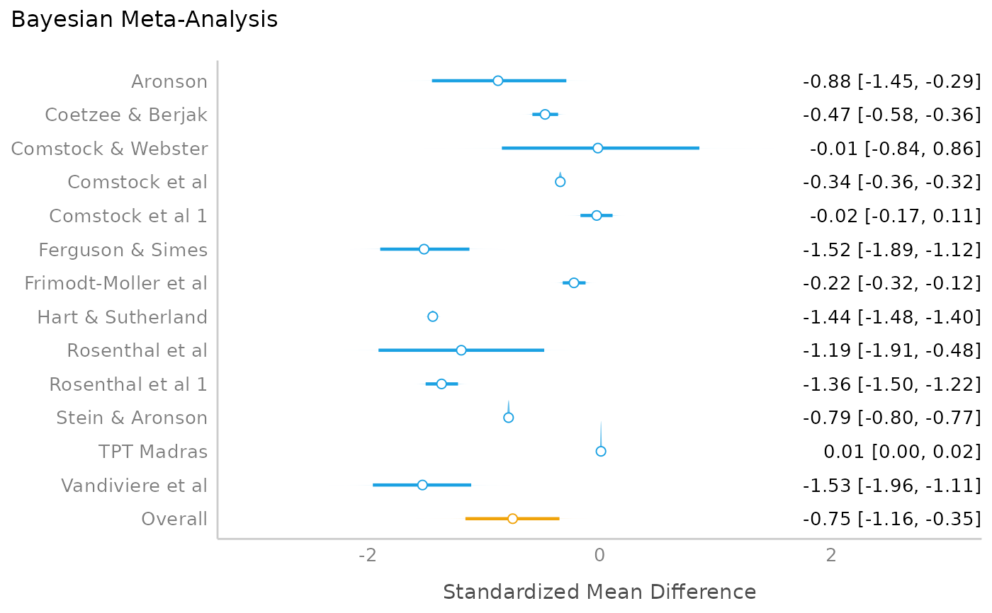
Plot method for Model Parameters from Bayesian Meta-Analysis

The plot() method for the parameters::model_parameters() function when used with brms-meta-analysis models.

Usage

# S3 method for class 'see_parameters_brms_meta'
plot(
  x,
  size_point = 2,
  size_line = 0.8,
  size_text = 3.5,
  posteriors_alpha = 0.7,
  rope_alpha = 0.15,
  rope_color = "cadetblue",
  normalize_height = TRUE,
  show_labels = TRUE,
  ...
)

Arguments

x

An object.

size_point

Numeric specifying size of point-geoms.

size_line

Numeric value specifying size of line geoms.

size_text

Numeric value specifying size of text labels.

posteriors_alpha

Numeric value specifying alpha for the posterior distributions.

rope_alpha

Numeric specifying transparency level of ROPE ribbon.

rope_color

Character specifying color of ROPE ribbon.

normalize_height

Logical. If TRUE, height of mcmc-areas is "normalized", to avoid overlap. In certain cases when the range of a posterior distribution is narrow for some parameters, this may result in very flat mcmc-areas. In such cases, set normalize_height = FALSE.

show_labels

Logical. If TRUE, text labels are displayed.

...

Arguments passed to or from other methods.

Value

A ggplot2-object.

Details

Colors of density areas and errorbars

To change the colors of the density areas, use scale_fill_manual() with named color-values, e.g. scale_fill_manual(values = c("Study" = "blue", "Overall" = "green")). To change the color of the error bars, use scale_color_manual(values = c("Errorbar" = "red")).

Show or hide estimates and CI

Use show_labels = FALSE to hide the textual output of estimates and credible intervals.

Examples

# \donttest{
library(parameters)
library(brms)
library(metafor)
data(dat.bcg)

dat <- escalc(
  measure = "RR",
  ai = tpos,
  bi = tneg,
  ci = cpos,
  di = cneg,
  data = dat.bcg
)
dat$author <- make.unique(dat$author)

# model
set.seed(123)
priors <- c(
  prior(normal(0, 1), class = Intercept),
  prior(cauchy(0, 0.5), class = sd)
)
model <- suppressWarnings(
  brm(yi | se(vi) ~ 1 + (1 | author), data = dat, refresh = 0, silent = 2)
)

# result
mp <- model_parameters(model)
plot(mp)

# }