Multilevel Correlations • correlation

This vignette can be cited as:

citation("correlation")

## To cite package 'correlation' in publications use:
## 
##   Makowski, D., Wiernik, B. M., Patil, I., Lüdecke, D., & Ben-Shachar,
##   M. S. (2022). correlation: Methods for correlation analysis (0.8.3)
##   [R package]. https://CRAN.R-project.org/package=correlation (Original
##   work published 2020)
## 
##   Makowski, D., Ben-Shachar, M. S., Patil, I., & Lüdecke, D. (2019).
##   Methods and algorithms for correlation analysis in R. Journal of Open
##   Source Software, 5(51), 2306. https://doi.org/10.21105/joss.02306
## 
## To see these entries in BibTeX format, use 'print(<citation>,
## bibtex=TRUE)', 'toBibtex(.)', or set
## 'options(citation.bibtex.max=999)'.

Data

Imagine we have an experiment in which 10 individuals completed a task with 100 trials. For each of the 1000 trials (10 * 100) in total, we measured two things, V1 and V2, and we are interested in investigating the link between these two variables.

We will generate data using the simulate_simpson() function from this package and look at its summary:

library(correlation)

data <- simulate_simpson(n = 100, groups = 10)

summary(data)

##        V1             V2           Group          
##  Min.   :-1.7   Min.   :-12.4   Length:1000       
##  1st Qu.: 3.0   1st Qu.: -8.0   Class :character  
##  Median : 5.6   Median : -5.5   Mode  :character  
##  Mean   : 5.5   Mean   : -5.5                     
##  3rd Qu.: 8.0   3rd Qu.: -3.0                     
##  Max.   :12.2   Max.   :  1.8

Now let’s visualize the two variables:

library(ggplot2)

ggplot(data, aes(x = V1, y = V2)) +
  geom_point() +
  geom_smooth(colour = "black", method = "lm", se = FALSE) +
  theme_classic()

## `geom_smooth()` using formula = 'y ~ x'

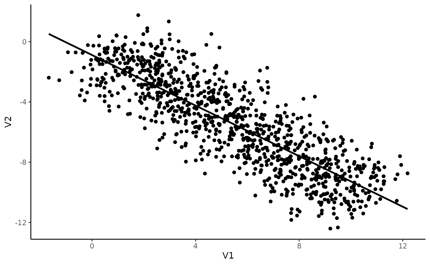
That seems pretty straightforward! It seems like there is a negative correlation between V1 and V2. Let’s test this.

Simple correlation

correlation(data)

## # Correlation Matrix (pearson-method)
## 
## Parameter1 | Parameter2 |     r |         95% CI | t(998) |         p
## ---------------------------------------------------------------------
## V1         |         V2 | -0.84 | [-0.86, -0.82] | -48.77 | < .001***
## 
## p-value adjustment method: Holm (1979)
## Observations: 1000

Indeed, there is a strong, negative and significant correlation between V1 and V2.

Great, can we go ahead and publish these results in PNAS?

The Simpson’s Paradox

Not so fast! Ever heard of the Simpson’s Paradox?

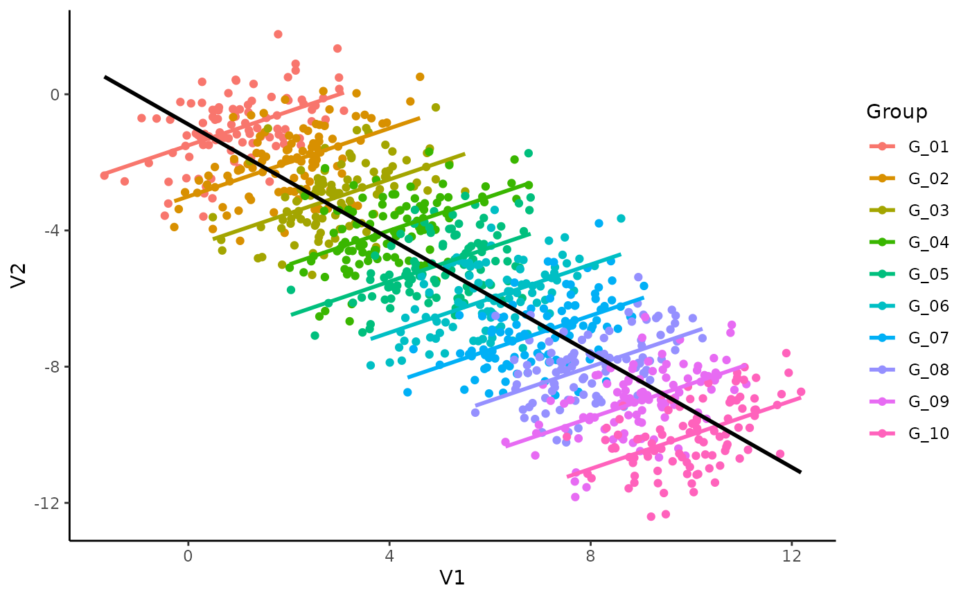
Let’s colour our datapoints by group (by individuals):

library(ggplot2)

ggplot(data, aes(x = V1, y = V2)) +
  geom_point(aes(colour = Group)) +
  geom_smooth(aes(colour = Group), method = "lm", se = FALSE) +
  geom_smooth(colour = "black", method = "lm", se = FALSE) +
  theme_classic()

## `geom_smooth()` using formula = 'y ~ x'
## `geom_smooth()` using formula = 'y ~ x'

Mmh, interesting. It seems like, for each subject, the relationship is different. The (global) negative trend seems to be an artifact of differences between the groups and could be spurious!

Multilevel (as in multi-group) correlations allow us to account for differences between groups. It is based on a partialization of the group, entered as a random effect in a mixed linear regression.

You can compute them with the correlations package by setting the multilevel argument to TRUE.

correlation(data, multilevel = TRUE)

## Parameter1 | Parameter2 |    r |           CI | t(998) |         p
## ------------------------------------------------------------------
## V1         |         V2 | 0.50 | [0.45, 0.55] |  18.24 | < .001***
## 
## Observations: 1000

For completeness, let’s also see if its Bayesian cousin agrees with it:

correlation(data, multilevel = TRUE, bayesian = TRUE)

## Parameter1 | Parameter2 |    r |           CI | t(998) |         p
## ------------------------------------------------------------------
## V1         |         V2 | 0.50 | [0.45, 0.54] |  18.12 | < .001***
## 
## Observations: 1000

Dayum! We were too hasty in our conclusions! Taking the group into account seems to be super important.

Note: In this simple case where only two variables are of interest, it would be of course best to directly proceed using a mixed regression model instead of correlations. That being said, the latter can be useful for exploratory analysis, when multiple variables are of interest, or in combination with a network or structural approach.