The goal of performance is to provide lightweight tools to assess and check the quality of your model. It includes functions such as r2() for many models (including logistic, mixed and Bayesian models), icc() or helpers to check_convergence(), check_overdipsersion() or check_zero-inflation() (see a complete list of functions here).
In this posting, we want to focus on multicollinearity. Multicollinearity “is a phenomenon in which one predictor variable in a multiple regression model can be linearly predicted from the others” (source), i.e. two or more predictors are more or less strongly correlated (also described as non-independent covariates). Multicollinearity may lead to severly biased regression coefficients and standard errors.
check_collinearity() checks your model predictors for collinearity. The function works for “simple” models, but also for mixed models, including zero-inflated mixed models fitted with the glmmTMB or GLMMadapative packages. The function provides a nice print() and plot() method, and examples are shown below.
Check Linear Models for Multicollinearity
First, we fit a simple linear model.
library(performance)

# fit model
data(mtcars)
model <- lm(mpg ~ wt + cyl + gear + disp, data = mtcars)
Now let’s check the model. Below you see two columns in the output, one indicating the variance inflation factor, VIF.
# now check for multicollinearity
check_collinearity(model)
## # Check for Multicollinearity
##
## Low Correlation
##
## Parameter VIF Increased SE
## gear 1.53 1.24
##
## Moderate Correlation
##
## Parameter VIF Increased SE
## wt 5.05 2.25
## cyl 5.41 2.33
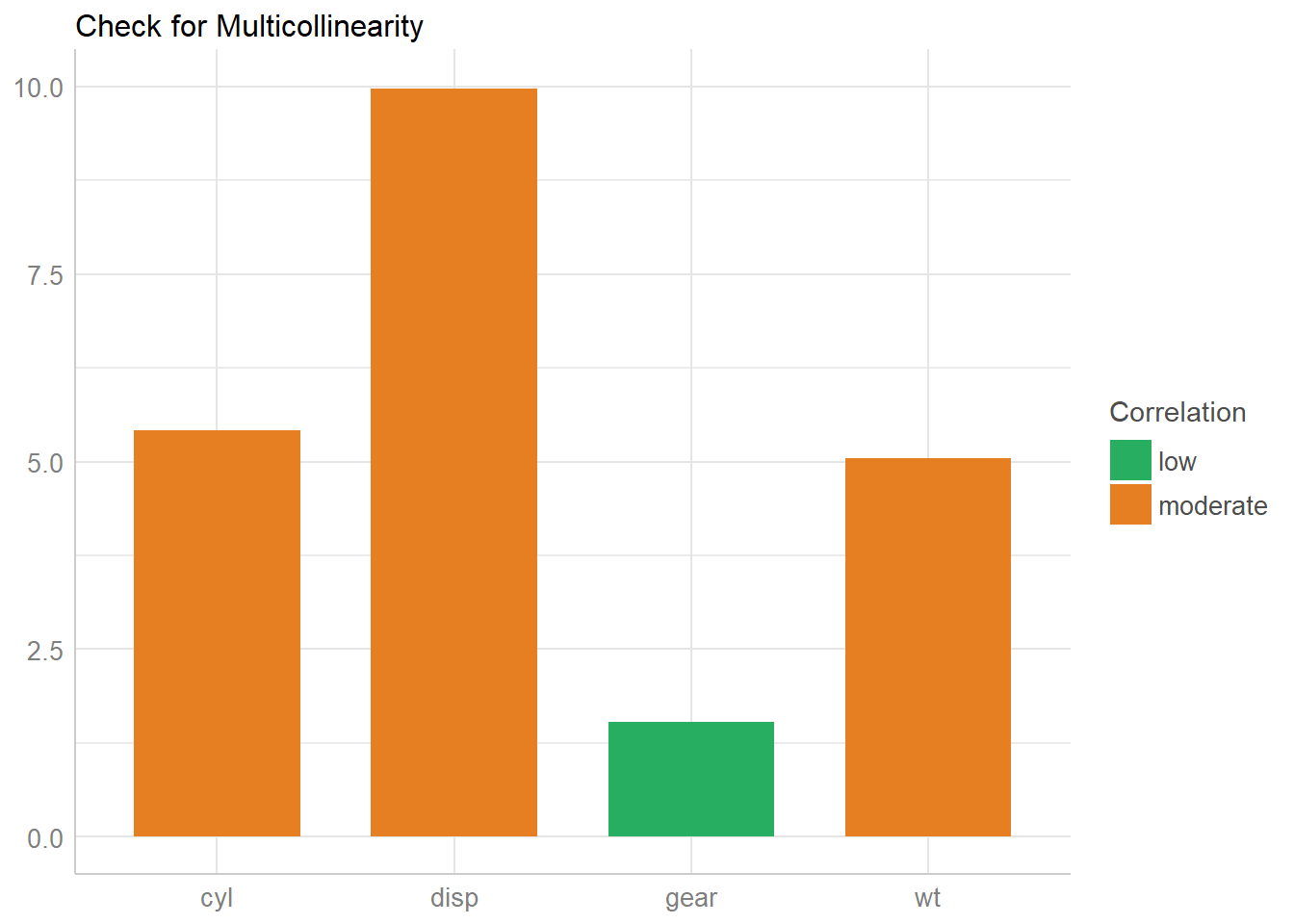
## disp 9.97 3.16The variance inflation factor is a measure to analyze the magnitude of multicollinearity of model terms. A VIF less than 5 indicates a low correlation of that predictor with other predictors. A value between 5 and 10 indicates a moderate correlation, while VIF values larger than 10 are a sign for high, not tolerable correlation of model predictors.
The Increased SE column in the output indicates how much larger the standard error is due to the correlation with other predictors.
Now let’s plot the results.
# plot results
x <- check_collinearity(model)
plot(x)
Check Zero-Inflated Mixed Models for Multicollinearity
For models with zero-inflation component, multicollinearity may happen both in the count as well as the zero-inflation component. By default, check_collinearity() checks the complete model, however, you can check only certain components of the model using the component-argument. In the following example, we will focus on the complete model.
library(glmmTMB)
data(Salamanders)

# create highly correlated pseudo-variable
set.seed(1)
Salamanders$cover2 <-
  Salamanders$cover * runif(n = nrow(Salamanders), min = .7, max = 1.3)

# fit mixed model with zero-inflation
model <- glmmTMB(
  count ~ spp + mined + cover + cover2 + (1 | site),
  ziformula = ~ spp + mined,
  family = truncated_poisson,
  data = Salamanders
)

# now check for multicollinearity
check_collinearity(model)
## # Check for Multicollinearity
##
## * conditional component:
##
## Low Correlation
##
## Parameter VIF Increased SE
## spp 1.07 1.04
## mined 1.17 1.08
##
## High Correlation
##
## Parameter VIF Increased SE
## cover 19.30 4.39
## cover2 19.12 4.37
##
## * zero inflated component:
##
## Low Correlation
##
## Parameter VIF Increased SE
## spp 1.08 1.04
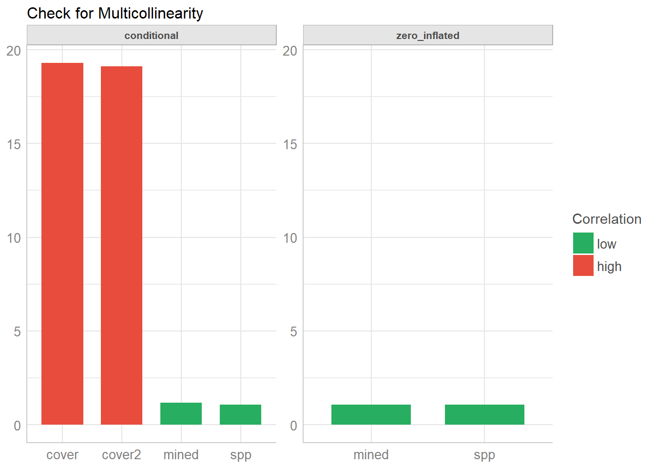
## mined 1.08 1.04As you can see, the print() method separates the results into the count and zero-inflated model components for a clearer output. Similar, plot() produces facets for each components, so it’s easier to understand.
plot(check_collinearity(model))
Remedies for Multicollinearity
Multicollinearity can have different reasons. Probably in many cases it will help to center or standardize the predictors. Sometimes the only way to avoid multicollinearity is to remove one of the predictors with a very high VIF value. Collecting more data may also help, but this is of course not always possible.
