The Problem with Null Effects
Say you fit an ANOVA model, predicting the time it takes to solve a puzzle from its shape (round / square) and whether it was colored or black and white, and you found that one of the estimated effects, in this case the interaction, was not significant. Say even that it was as non-significant as can be, with p = 1.00!
options(contrasts = c('contr.sum', 'contr.poly'))

data("puzzles", package = "BayesFactor")
aov_model <- aov(RT ~ shape*color + Error(ID/(shape*color)), data = puzzles)

summary(aov_model)
##
## Error: ID
## Df Sum Sq Mean Sq F value Pr(>F)
## Residuals 11 226 20.6
##
## Error: ID:shape
## Df Sum Sq Mean Sq F value Pr(>F)
## shape 1 12.0 12.00 7.54 0.019 *
## Residuals 11 17.5 1.59
## ---
## Signif. codes: 0 '***' 0.001 '**' 0.01 '*' 0.05 '.' 0.1 ' ' 1
##
## Error: ID:color
## Df Sum Sq Mean Sq F value Pr(>F)
## color 1 12.0 12.00 13.9 0.0033 **
## Residuals 11 9.5 0.86
## ---
## Signif. codes: 0 '***' 0.001 '**' 0.01 '*' 0.05 '.' 0.1 ' ' 1
##
## Error: ID:shape:color
## Df Sum Sq Mean Sq F value Pr(>F)
## shape:color 1 0.0 0.00 0 1
## Residuals 11 30.5 2.77You look at your data, as you were taught to do, and it really does seems like the effect of color is not moderated by shape (and vice versa):
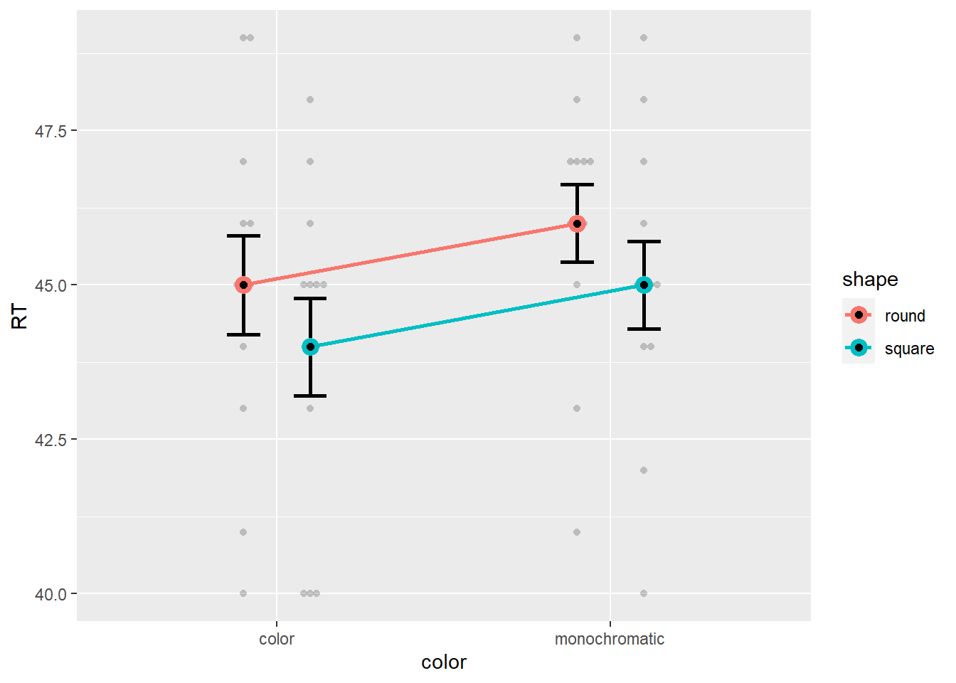
But what does this mean? Can you infer that there isn’t interaction? Are the two simple effects of color truly identical?
Classical statistics has no answer for us here - when the p-value is less than alpha (typically 5%) we can reject the null hypothesis, but when p > .05, even a lot bigger than 5%, classical (frequentists) statistics do not allow to infer that the null is true. For this, we need to go Bayesian!
Going Bayesian
One of the (many) strengths of Bayesian statistics is its ability to support the null hypothesis. Let us fit a Bayesian mixed model equivalent to the repeated measures ANOVA above, manually specifying weakly informative priors on its effects:
library(rstanarm)
stan_model <- stan_lmer(RT ~ shape*color + (1 | ID), data = puzzles,
                        prior = cauchy(0,c(0.707,0.707,0.5),          # as per Rouder et al., 2012
                        prior_intercept = student_t(3,0,10),          # weakly informative
                        prior_aux = exponential(.1),                  # weakly informative
                        prior_covariance = decov(1,1,1,1))            # weakly informative
Using the fantastic emmeans package, we can explore and extract marginal effects and estimates from our fitted model. For example, we can estimate the main effect for color:
c_color_main <- pairs(emmeans(stan_model, ~ color))
c_color_main
## contrast estimate lower.HPD upper.HPD
## color - monochromatic -0.894 -1.67 -0.147
##
## Point estimate displayed: median
## HPD interval probability: 0.95We can also estimate (based on posterior draws) the difference between the two simple effects for color between the levels of shape:
em_color_simple <- emmeans(stan_model, ~color * shape)
pairs(em_color_simple, by = "shape") # simple effects for color
## shape = round:
## contrast estimate lower.HPD upper.HPD
## color - monochromatic -0.898 -1.96 0.107
##
## shape = square:
## contrast estimate lower.HPD upper.HPD
## color - monochromatic -0.887 -1.89 0.212
##
## Point estimate displayed: median
## HPD interval probability: 0.95c_color_shape_interaction <- contrast(em_color_simple, interaction = c("pairwise","pairwise"))
c_color_shape_interaction## color_pairwise shape_pairwise estimate lower.HPD upper.HPD
## color - monochromatic round - square 0.0108 -1.36 1.38
##
## Point estimate displayed: median
## HPD interval probability: 0.95As we can see, the simple effects are indeed similar, and the difference between them seems very close to 0. Can we quantify the evidence for the null?
Quantifying Evidence for the Null
One way to quantify evidence in the Bayesian framework is to calculate a Bayes factor - a measure of relative evidence in favor of one model over another. In our case, we would like to compare a model with an interaction to a model without an interaction. Though we could fit the model without the interaction and compare the two with bayesfactor_models(), we’ll use a close approximation using the Savage-Dickey density ratio, which allows for more flexibility. To this end we can use (from version 0.2.1, available on GitHub) describe_posterior() to… well… describe our emmeans estimates’ posterior distribution, and by comparing the density of the null value (here 0) between the prior and posterior, we can compute the Savage-Dickey Bayes factor! (Note that we will need to pass the original model via bf_prior to allow the extraction or prior draw.)
# combine all estimates of interest to one object:
c_color_all <- rbind(c_color_main,
                     c_color_shape_interaction)
c_color_all
## contrast color_pairwise shape_pairwise estimate lower.HPD
## color - monochromatic . . -0.894 -1.67
## . color - monochromatic round - square 0.011 -1.36
## upper.HPD
## -0.147
## 1.378
##
## Point estimate displayed: median
## HPD interval probability: 0.95describe_posterior(c_color_all,
estimate = "median", dispersion = TRUE,
ci = .9, ci_method = "hdi",
test = c("bayesfactor"),
bf_prior = stan_model)| Parameter | Median | MAD | CI | CI_low | CI_high | BF | |
|---|---|---|---|---|---|---|---|
| 2 | color - monochromatic, ., . | -0.894 | 0.395 | 90 | -1.50 | -0.227 | 3.128 |
| 1 | ., color - monochromatic, round - square | 0.011 | 0.700 | 90 | -1.16 | 1.145 | 0.272 |
These Bayes factors reveal that a model with a main effect for color is ~3 times more likely than a model without this effect, and that a model without an interaction is ~1/0.22 = 4.5 times more likely than a model with an interaction! But… note that a Bayes factor of 4.5 is considered only moderate evidence in favor of the null effect. As we can see, a p-value of 1.0 does not necessarily mean the data strongly supports the null.
Happy Bayesing!