The p-direction: A Bayesian equivalent of the p-value?

Feb 26, 2020 in BAYESTESTR • R
r easystats bayestestr p-value pd p-direction
4 min read

The Bayesian framework is powerful and allows for an incredible amount of flexibility and control over your analysis. That being said, newcomers often struggle with a lot of new concepts and tools and could benefit from some familiar grounding. And the p-value is a very familiar index (although paradoxically often misunderstood, but that’s another topic).

Is there an equivalent of the p-value? Well, depends on what “equivalent” means. Some might argue that the Bayes factor is some sort of equivalent, i.e., a value that can be used for decisions and interpretation of results. Some others would suggest that the MAP-based p-value is another alternative.

Based on a simulation study (Makowski et al., 2019), we think that the probability of direction (p-direction, or pd) is the closest statistical equivalent to the p-value. The statistical is important here, simply meaning that the two indices are strongly correlated. That being said, they are not conceptually equivalent (as we argue in the paper, the pd is an index of effect existence, rather than significance).

Here’s a short example.

Frequentist regression

First, you can install (or update) the necessary packages by running the following (it’s important that the insight package version must be >= 0.8.1):

install.packages(c("insight", "bayestestR", "parameters"))

Let’s start by running a simple linear regression and displaying its result with the parameters package.

library(parameters)

model <- lm(disp ~ carb, data = mtcars)
parameters(model)

## Parameter   | Coefficient |    SE |          95% CI | t(30) |     p
## -------------------------------------------------------------------
## (Intercept) |      145.48 | 41.58 | [60.56, 230.40] |  3.50 | 0.001
## carb        |       30.31 | 12.87 | [ 4.02,  56.59] |  2.35 | 0.025

The p-value of the linear relationship between the two variable is of .025 (the second row in the p column). What does a Bayesian analysis tells us?

Bayesian regression (with flat priors)

As you might know, a Bayesian analysis is close to a maximum likelihood analysis (the typical frequentist paradigm) when no information is given by the prior (and the result is only driven by the data). This is the case with flat priors, that give equivalent likelihood to each and every one of your wildest dreams (see the How to Specify Flat Priors (and why you typically shouldn’t) section).

Let’s fit the same regression as above within a Bayesian framework with a flat prior (i.e., by setting them as NULL).

library(bayestestR)
library(rstanarm)

model <-
  stan_glm(
    disp ~ carb,
    data = mtcars,
    priors = NULL,
    prior_intercept = NULL
  )

parameters(model)

## Parameter   | Median |          89% CI |     pd | % in ROPE |  Rhat |   ESS |                Prior
## --------------------------------------------------------------------------------------------------
## (Intercept) | 145.87 | [77.91, 215.41] | 99.94% |     0.14% | 1.000 | 52545 |       Uniform ( +- )
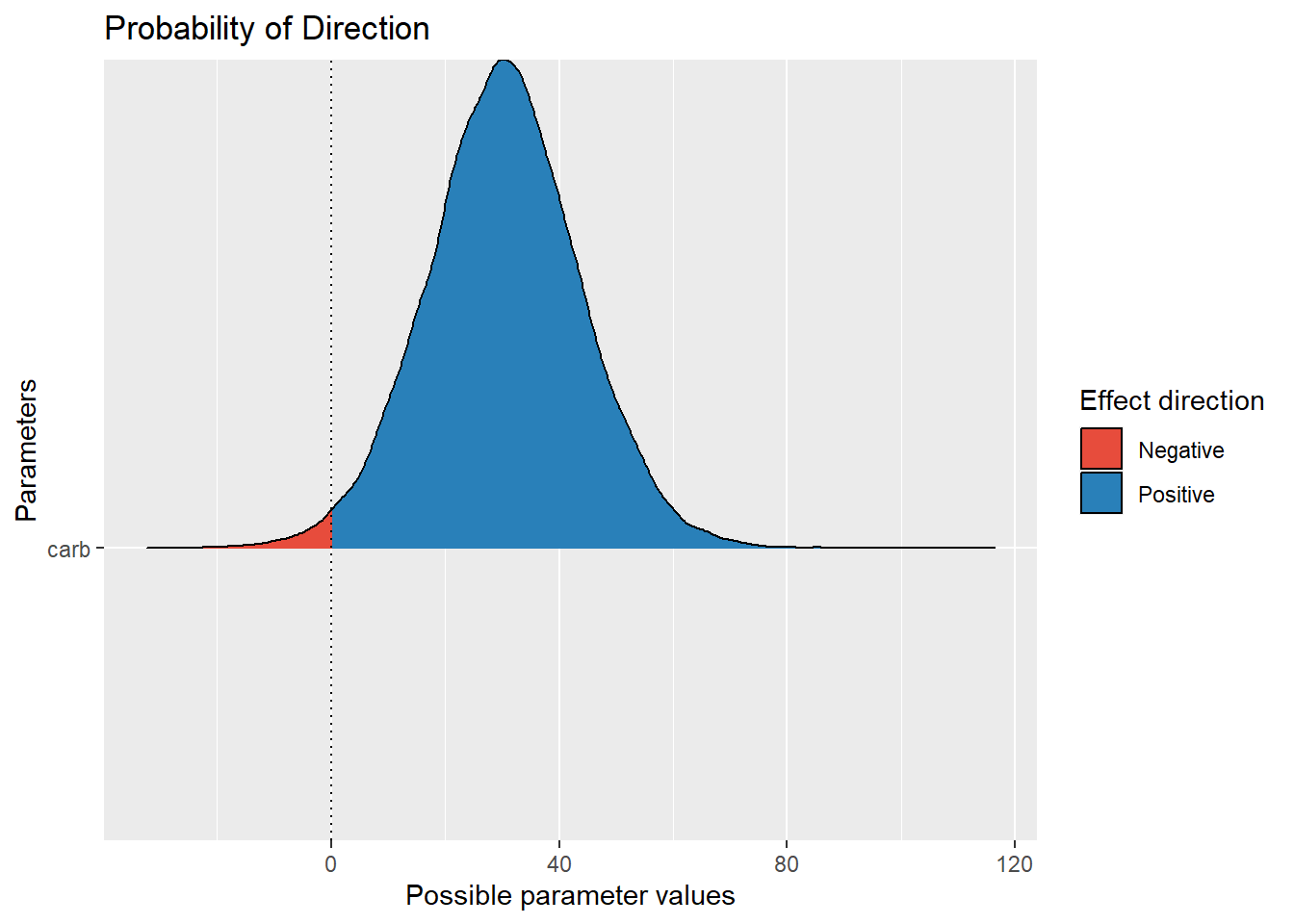
## carb        |  30.22 | [ 9.10,  51.92] | 98.68% |     8.89% | 1.000 | 52711 | Normal (0 +- 191.83)

It tells us that the p-direction is of 98.80%, i.e., 0.9880 (note that your results can slightly vary due to the random nature of the sampling; you can increase the number of iterations to get more stable results). We can quickly visualize its meaning as follows (with the see package):

library(see)

plot(p_direction(model))

From p-direction to p-value

We can convert this value to a p-value using the following function:

pd_to_p(0.9880)

## [1] 0.024

As we can see, we are not far from the frequentist p-value!

But again, we need to underline that the p-direction has a different meaning and interpretation. It refers to the probability that the effect is positive or negative (depending on the median’s sign). But like the p-value, it cannot either be used to support a lack of an effect (for that, ROPE-based indices or Bayes factors might be more appropriate).

Moreover, when using informative priors centred at 0, a Bayesian analysis will always lead to “less significant” effects, as the prior will pull the posterior towards 0. This is a natural way of penalizing results, which is a good thing.

In conclusion, make sure you understand the indices you use (for instance by checking-out our gentle intro to Bayesian analysis)!

Get Involved

easystats is a new project in active development, looking for contributors and supporters. Thus, do not hesitate to contact us if you want to get involved :)

Check out our other blog posts here!

Stay tuned

To be updated about the upcoming features and cool R or data science stuff, you can follow the packages on GitHub (click on one of the easystats package) and then on the Watch button on the top right corner) as well as the easystats team on twitter and online: