![]()
The correlation package
The easystats project continues to grow with its more recent addition, a package devoted to correlations. Check-out its webpage here!
It’s lightweight, easy to use, and allows for the computation of many different kinds of correlations, such as partial correlations, Bayesian correlations, multilevel correlations, polychoric correlations, biweight, percentage bend or Sheperd’s Pi correlations (types of robust correlation), distance correlation (a type of non-linear correlation) and more, also allowing for combinations between them (for instance, Bayesian partial multilevel correlation).
You can install and load the package as follows:
install.packages("correlation")
library(correlation)
Examples
The main function is correlation(), which builds on top of cor_test() and comes with a number of possible options.
Correlation details and matrix
cor <- correlation(iris)
cor
## Parameter1 | Parameter2 | r | 95% CI | t(148) | p | Method | n_Obs
## ----------------------------------------------------------------------------------------
## Sepal.Length | Sepal.Width | -0.12 | [-0.27, 0.04] | -1.44 | 0.152 | Pearson | 150
## Sepal.Length | Petal.Length | 0.87 | [ 0.83, 0.91] | 21.65 | < .001 | Pearson | 150
## Sepal.Length | Petal.Width | 0.82 | [ 0.76, 0.86] | 17.30 | < .001 | Pearson | 150
## Sepal.Width | Petal.Length | -0.43 | [-0.55, -0.29] | -5.77 | < .001 | Pearson | 150
## Sepal.Width | Petal.Width | -0.37 | [-0.50, -0.22] | -4.79 | < .001 | Pearson | 150
## Petal.Length | Petal.Width | 0.96 | [ 0.95, 0.97] | 43.39 | < .001 | Pearson | 150
##
## p-value adjustment method: Holm (1979)The output is not a square matrix, but a (tidy) dataframe with all correlations tests per row. One can also obtain a matrix using:
summary(cor)## Parameter | Petal.Width | Petal.Length | Sepal.Width
## -------------------------------------------------------
## Sepal.Length | 0.82*** | 0.87*** | -0.12
## Sepal.Width | -0.37*** | -0.43*** |
## Petal.Length | 0.96*** | |Note that one can also obtain the full, square and redundant matrix using:
as.table(cor)## Parameter | Sepal.Length | Sepal.Width | Petal.Length | Petal.Width
## ----------------------------------------------------------------------
## Sepal.Length | 1.00*** | -0.12 | 0.87*** | 0.82***
## Sepal.Width | -0.12 | 1.00*** | -0.43*** | -0.37***
## Petal.Length | 0.87*** | -0.43*** | 1.00*** | 0.96***
## Petal.Width | 0.82*** | -0.37*** | 0.96*** | 1.00***Grouped dataframes
The function also supports stratified correlations, all within the tidyverse workflow!
library(dplyr)

iris %>%
  select(Species, Petal.Width, Sepal.Length, Sepal.Width) %>%
  group_by(Species) %>%
  correlation()
## Group | Parameter1 | Parameter2 | r | 95% CI | t(48) | p | Method | n_Obs
## --------------------------------------------------------------------------------------------------
## setosa | Petal.Width | Sepal.Length | 0.28 | [ 0.00, 0.52] | 2.01 | 0.101 | Pearson | 50
## setosa | Petal.Width | Sepal.Width | 0.23 | [-0.05, 0.48] | 1.66 | 0.104 | Pearson | 50
## setosa | Sepal.Length | Sepal.Width | 0.74 | [ 0.59, 0.85] | 7.68 | < .001 | Pearson | 50
## versicolor | Petal.Width | Sepal.Length | 0.55 | [ 0.32, 0.72] | 4.52 | < .001 | Pearson | 50
## versicolor | Petal.Width | Sepal.Width | 0.66 | [ 0.47, 0.80] | 6.15 | < .001 | Pearson | 50
## versicolor | Sepal.Length | Sepal.Width | 0.53 | [ 0.29, 0.70] | 4.28 | < .001 | Pearson | 50
## virginica | Petal.Width | Sepal.Length | 0.28 | [ 0.00, 0.52] | 2.03 | 0.048 | Pearson | 50
## virginica | Petal.Width | Sepal.Width | 0.54 | [ 0.31, 0.71] | 4.42 | < .001 | Pearson | 50
## virginica | Sepal.Length | Sepal.Width | 0.46 | [ 0.20, 0.65] | 3.56 | 0.002 | Pearson | 50
##
## p-value adjustment method: Holm (1979)Bayesian Correlations
It is very easy to switch to a Bayesian framework.
correlation(iris, bayesian=TRUE)## Parameter1 | Parameter2 | rho | 95% CI | pd | % in ROPE | BF | Prior | Method | n_Obs
## -----------------------------------------------------------------------------------------------------------------------------
## Sepal.Length | Sepal.Width | -0.11 | [-0.25, 0.02] | 90.77% | 44.17% | 0.509 | Beta (3 +- 3) | Bayesian Pearson | 150
## Sepal.Length | Petal.Length | 0.86 | [ 0.83, 0.89] | 100% | 0% | > 1000 | Beta (3 +- 3) | Bayesian Pearson | 150
## Sepal.Length | Petal.Width | 0.80 | [ 0.76, 0.85] | 100% | 0% | > 1000 | Beta (3 +- 3) | Bayesian Pearson | 150
## Sepal.Width | Petal.Length | -0.41 | [-0.52, -0.30] | 100% | 0% | > 1000 | Beta (3 +- 3) | Bayesian Pearson | 150
## Sepal.Width | Petal.Width | -0.35 | [-0.47, -0.24] | 100% | 0.02% | > 1000 | Beta (3 +- 3) | Bayesian Pearson | 150
## Petal.Length | Petal.Width | 0.96 | [ 0.95, 0.97] | 100% | 0% | > 1000 | Beta (3 +- 3) | Bayesian Pearson | 150Tetrachoric, Polychoric, Biserial, Biweight…
The correlation package also supports different types of methods, which can deal with correlations between factors!
correlation(iris, include_factors = TRUE, method = "auto")## Parameter1 | Parameter2 | r | 95% CI | t(148) | p | Method | n_Obs
## -----------------------------------------------------------------------------------------------------------
## Sepal.Length | Sepal.Width | -0.12 | [-0.27, 0.04] | -1.44 | 0.452 | Pearson | 150
## Sepal.Length | Petal.Length | 0.87 | [ 0.83, 0.91] | 21.65 | < .001 | Pearson | 150
## Sepal.Length | Petal.Width | 0.82 | [ 0.76, 0.86] | 17.30 | < .001 | Pearson | 150
## Sepal.Length | Species.setosa | -0.72 | [-0.79, -0.63] | -12.53 | < .001 | Point-biserial | 150
## Sepal.Length | Species.versicolor | 0.08 | [-0.08, 0.24] | 0.97 | 0.452 | Point-biserial | 150
## Sepal.Length | Species.virginica | 0.64 | [ 0.53, 0.72] | 10.08 | < .001 | Point-biserial | 150
## Sepal.Width | Petal.Length | -0.43 | [-0.55, -0.29] | -5.77 | < .001 | Pearson | 150
## Sepal.Width | Petal.Width | -0.37 | [-0.50, -0.22] | -4.79 | < .001 | Pearson | 150
## Sepal.Width | Species.setosa | 0.60 | [ 0.49, 0.70] | 9.20 | < .001 | Point-biserial | 150
## Sepal.Width | Species.versicolor | -0.47 | [-0.58, -0.33] | -6.44 | < .001 | Point-biserial | 150
## Sepal.Width | Species.virginica | -0.14 | [-0.29, 0.03] | -1.67 | 0.392 | Point-biserial | 150
## Petal.Length | Petal.Width | 0.96 | [ 0.95, 0.97] | 43.39 | < .001 | Pearson | 150
## Petal.Length | Species.setosa | -0.92 | [-0.94, -0.89] | -29.13 | < .001 | Point-biserial | 150
## Petal.Length | Species.versicolor | 0.20 | [ 0.04, 0.35] | 2.51 | 0.066 | Point-biserial | 150
## Petal.Length | Species.virginica | 0.72 | [ 0.63, 0.79] | 12.66 | < .001 | Point-biserial | 150
## Petal.Width | Species.setosa | -0.89 | [-0.92, -0.85] | -23.41 | < .001 | Point-biserial | 150
## Petal.Width | Species.versicolor | 0.12 | [-0.04, 0.27] | 1.44 | 0.452 | Point-biserial | 150
## Petal.Width | Species.virginica | 0.77 | [ 0.69, 0.83] | 14.66 | < .001 | Point-biserial | 150
## Species.setosa | Species.versicolor | -0.88 | [-0.91, -0.84] | -22.43 | < .001 | Tetrachoric | 150
## Species.setosa | Species.virginica | -0.88 | [-0.91, -0.84] | -22.43 | < .001 | Tetrachoric | 150
## Species.versicolor | Species.virginica | -0.88 | [-0.91, -0.84] | -22.43 | < .001 | Tetrachoric | 150
##
## p-value adjustment method: Holm (1979)Partial Correlations
It also supports partial correlations:
iris %>%
  correlation(partial = TRUE) %>%
  summary()
## Parameter | Petal.Width | Petal.Length | Sepal.Width
## -------------------------------------------------------
## Sepal.Length | -0.34*** | 0.72*** | 0.63***
## Sepal.Width | 0.35*** | -0.62*** |
## Petal.Length | 0.87*** | |Gaussian Graphical Models (GGMs)
Such partial correlations can also be represented as Gaussian graphical models, an increasingly popular tool in psychology:
library(see) # for plotting
library(ggraph) # needs to be loaded

mtcars %>%
  correlation(partial = TRUE) %>%
  plot()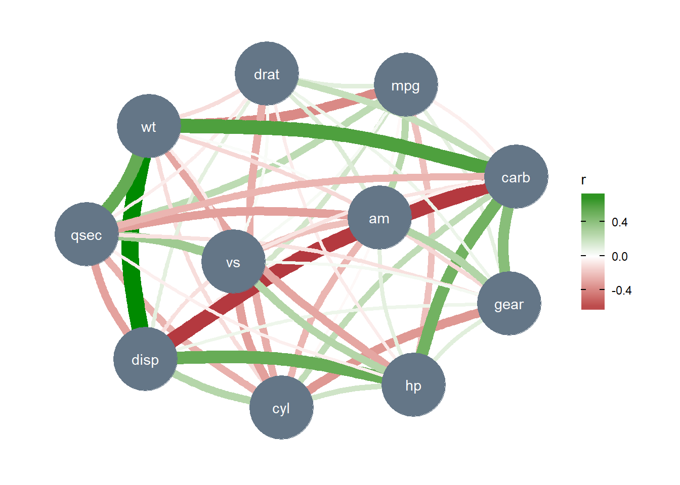
Get Involved
easystats is a new project in active development, looking for contributors and supporters. Thus, do not hesitate to contact us if you want to get involved :)
- Check out our other blog posts here!
Stay tuned
To be updated about the upcoming features and cool R or data science stuff, you can follow the packages on GitHub (click on one of the easystats package) and then on the Watch button on the top right corner) as well as the easystats team on twitter and online: