
New Features of the parameters and see Package
We’re excited to announce some news from the easystats-project. Two packages were updated recently, the parameters-package and our visualization-toolbox, the see-package.
Before we start introducing some of the new features, we’d like to explain why you need the see-package to create plots for functions from other easystats packages. So, the see-package not only includes additional geoms, color scales and themes for ggplot2, but - maybe more important - also provides plot()-methods for many functions from the various easystats packages. By separating the plotting functionality from our core packages, packages from the easystats-project don’t rely nor import any other packages! This means that you can safely use them as dependencies in your own packages, without the risk of butterfly effects (a small change in a distant downstream dependency with unexpected upstream consequences).
Print and Plot your Model Parameters
The model_parameters() function in the parameters-package is simlar to broom::tidy() - it returns a summary of the model parameters as a clean, consistent data frame. standardize_names() can be used to return a data frame with column names as they are used in other packages (like broom).
model_parameters() supports many different models, including mixed or Bayesian regression models. It comes with nice print() and plot() methods.
Examples - Zero Inflated Mixed Models with glmmTMB
The first example is a zero-inflated mixed model, fitted with the glmmTMB-package. model_parameters() creates separate tables for different model components (like zero-inflated components).
library(glmmTMB)
data(Salamanders)
model <- glmmTMB(
  count ~ spp + mined + (1 | site),
  ziformula = ~mined,
  family = poisson(),
  data = Salamanders
)

model_parameters(model)
## # Fixed Effects
##
## Parameter | Log-Mean | SE | 95% CI | z | p
## ---------------------------------------------------------------
## (Intercept) | -0.36 | 0.28 | [-0.90, 0.18] | -1.30 | 0.194
## spp [PR] | -1.27 | 0.24 | [-1.74, -0.80] | -5.27 | < .001
## spp [DM] | 0.27 | 0.14 | [ 0.00, 0.54] | 1.95 | 0.051
## spp [EC-A] | -0.57 | 0.21 | [-0.97, -0.16] | -2.75 | 0.006
## spp [EC-L] | 0.67 | 0.13 | [ 0.41, 0.92] | 5.20 | < .001
## spp [DES-L] | 0.63 | 0.13 | [ 0.38, 0.87] | 4.96 | < .001
## spp [DF] | 0.12 | 0.15 | [-0.17, 0.40] | 0.78 | 0.435
## mined [no] | 1.27 | 0.27 | [ 0.74, 1.80] | 4.72 | < .001
##
## # Zero-Inflated
##
## Parameter | Log-Odds | SE | 95% CI | z | p
## ---------------------------------------------------------------
## (Intercept) | 0.79 | 0.27 | [ 0.26, 1.32] | 2.90 | 0.004
## mined [no] | -1.84 | 0.31 | [-2.46, -1.23] | -5.87 | < .001If only a specific part of the model should be shown, use the component-argument.
model_parameters(model, component = "zero_inflated")## Parameter | Log-Mean | SE | 95% CI | z | p
## ---------------------------------------------------------------
## (Intercept) | 0.79 | 0.27 | [ 0.26, 1.32] | 2.90 | 0.004
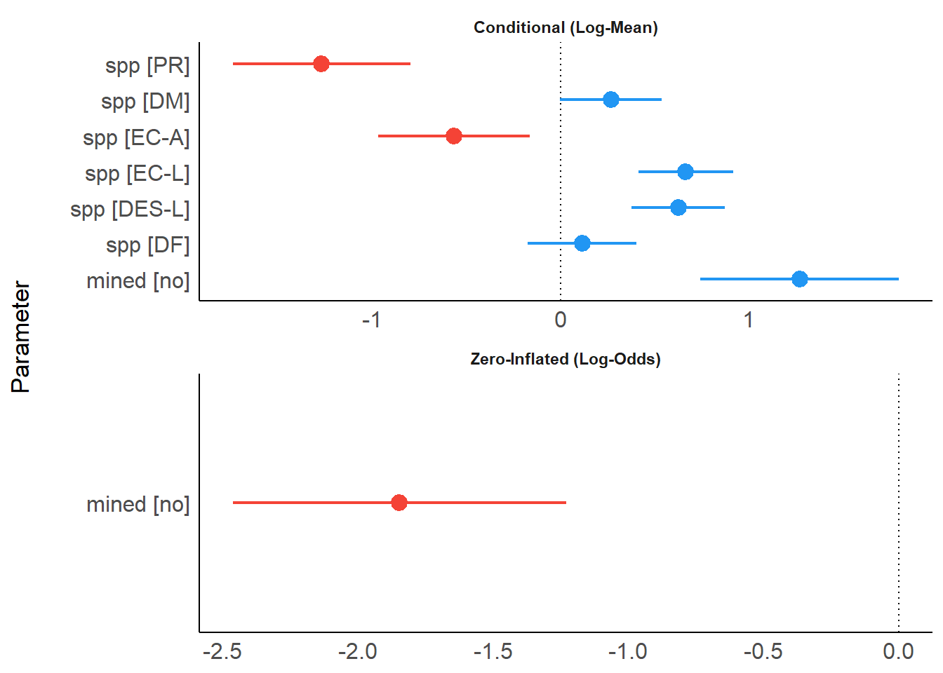
## mined [no] | -1.84 | 0.31 | [-2.46, -1.23] | -5.87 | < .001plot() creates a so called “forest plot”. In case of models with multiple components, parameters are separated into facets by model component.
result <- model_parameters(model)
plot(result)
Examples - Bayesian Mixed Models with brms
For the next example, we download a pre-compiled brms model to save computation time. For Bayesian models, by default, only “fixed” effects are shown. Using effects = "all" and component = "all" allows us to display random effects and the parameters of the zero-inflated model part as well.
# We download the model to save computation time. Here is the code
# to refit the exact model used below...

# zinb <- read.csv("http://stats.idre.ucla.edu/stat/data/fish.csv")
# set.seed(123)
# model <- brm(bf(
#     count ~ persons + child + camper + (1 | persons),
#     zi ~ child + camper + (1 | persons)
#   ),
#   data = zinb,
#   family = zero_inflated_poisson()
# )
brms_model <- insight::download_model("brms_zi_2")
result <- model_parameters(brms_model, effects = "all", component = "all")

result
## Parameter | Median | 89% CI | pd | % in ROPE | Rhat | ESS
## -------------------------------------------------------------------------
## (Intercept) | -0.86 | [-1.37, -0.34] | 98.22% | 1.30% | 1.002 | 1003
## persons | 0.84 | [ 0.68, 1.01] | 100% | 0% | 1.002 | 878
## child | -1.15 | [-1.29, -1.00] | 100% | 0% | 1.001 | 2166
## camper | 0.73 | [ 0.58, 0.89] | 100% | 0% | 1.000 | 3528
##
## Parameter | Median | 89% CI | pd | % in ROPE | Rhat | ESS
## -------------------------------------------------------------------------
## (Intercept) | -0.65 | [-1.82, 0.47] | 83.17% | 7.80% | 1.000 | 1174
## child | 1.86 | [ 1.37, 2.42] | 100% | 0% | 1.002 | 3022
## camper | -0.84 | [-1.40, -0.24] | 98.95% | 1.68% | 1.000 | 3410
##
## Parameter | Median | 89% CI | pd | % in ROPE | Rhat | ESS
## --------------------------------------------------------------------
## (Intercept) | 0.12 | [0.00, 0.39] | 100% | 45.27% | 1.005 | 819
##
## Parameter | Median | 89% CI | pd | % in ROPE | Rhat | ESS
## ---------------------------------------------------------------------
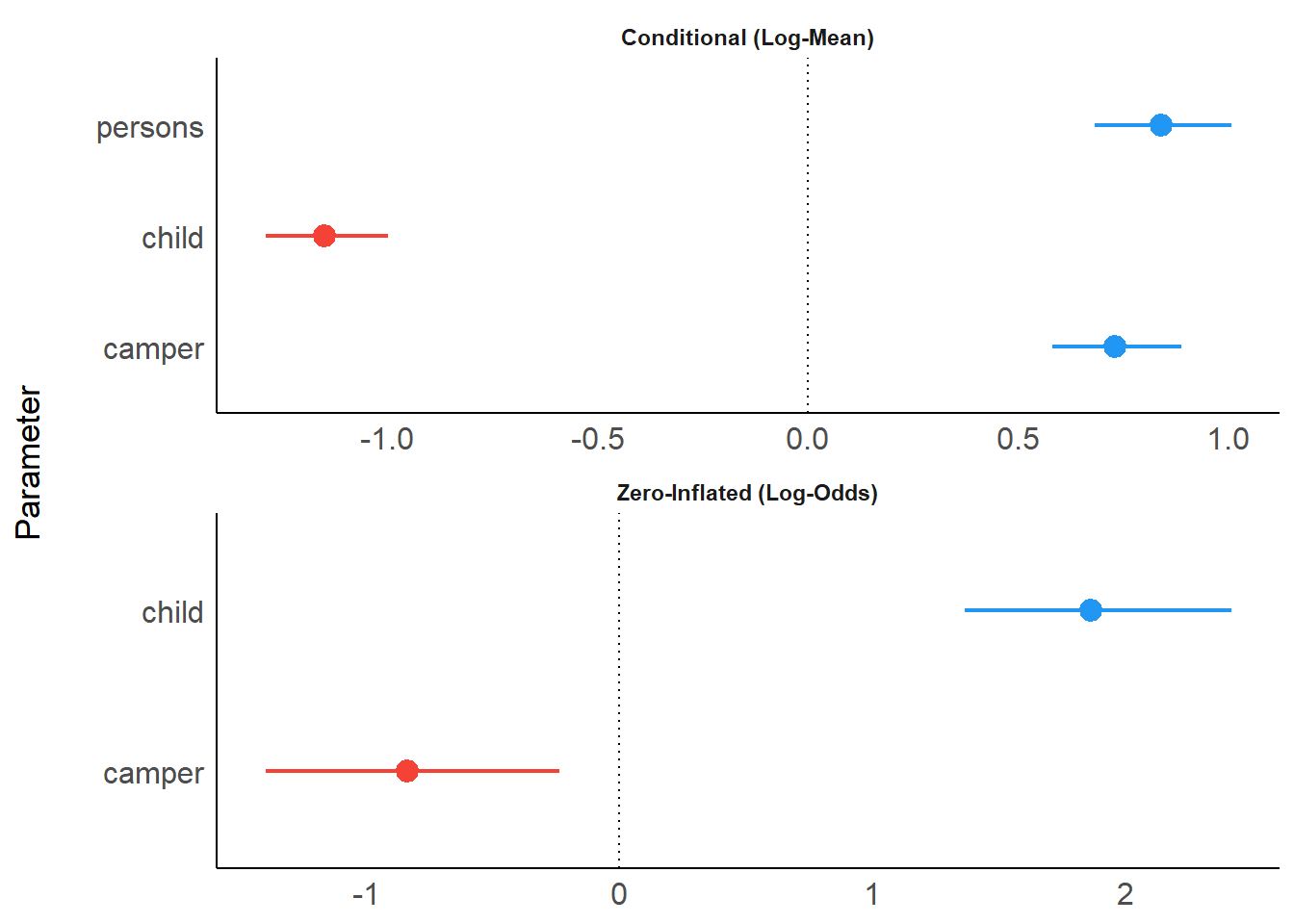
## (Intercept) | 1.32 | [0.48, 2.49] | 100% | 0% | 1.004 | 1331plot() now creates four facets by default. Note that plots from the parameters-package create forest plots. If you prefer plots that show the complete posterior distribution, you may rather use functions from the bayestestRR-package, as shown here.
plot(result)
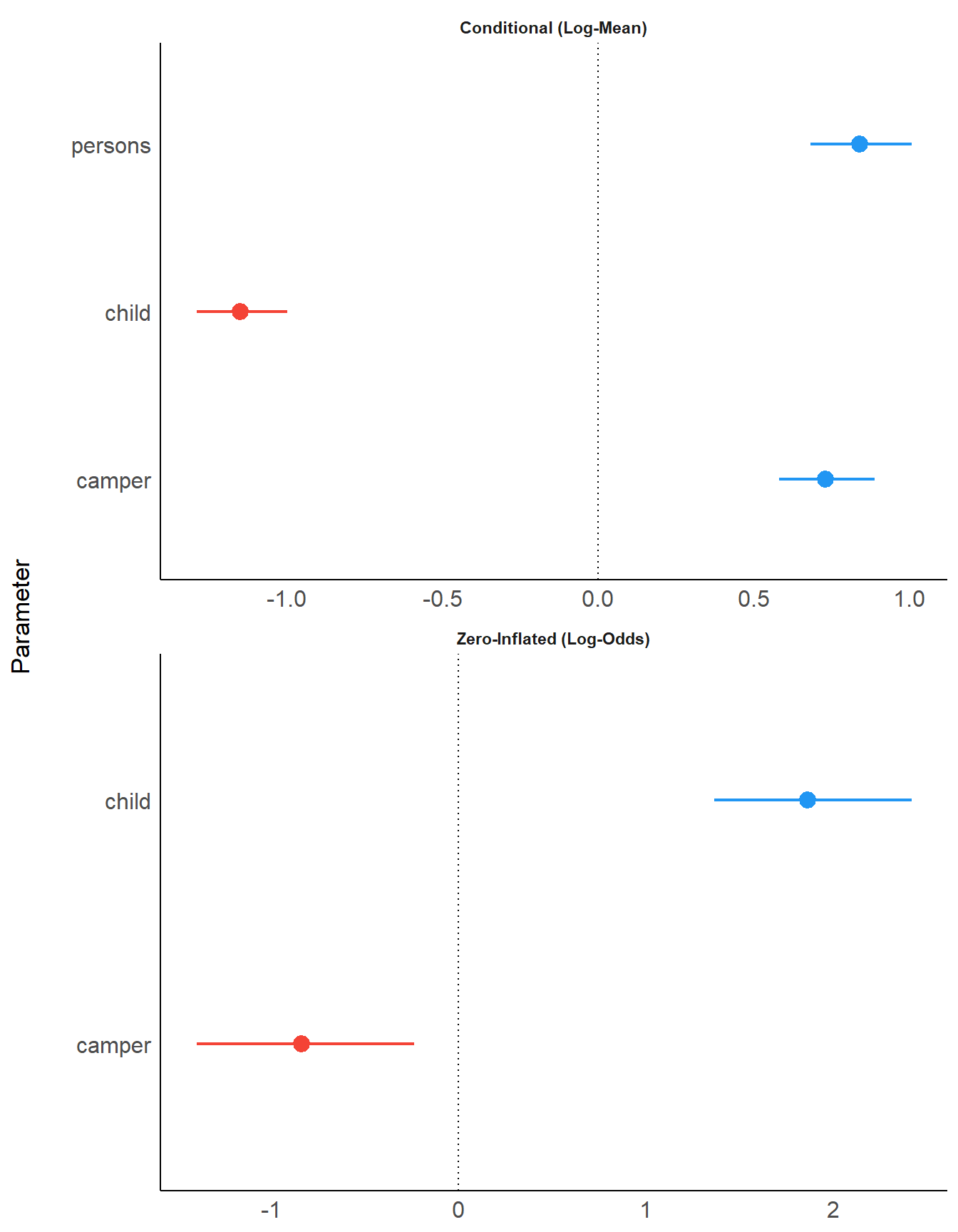
You can modify the layout with n_columns.
plot(result, n_columns = 1)
Examples - Meta-Analysis with metafor
Even results from meta-analyses, using the metafor-package, can be visualized with parameters and see.
library(metafor)
d <- data.frame(
  effectsize = c(-0.393, 0.675, 0.282, -1.398),
  standarderror = c(0.317, 0.317, 0.13, 0.36)
)

ma <- rma(yi = effectsize, sei = standarderror, method = "REML", data = d)
result <- model_parameters(ma)

result
## # Meta-analysis using 'metafor'
##
## Parameter | Coefficient | SE | 95% CI | z | p | Weight
## -------------------------------------------------------------------------
## Study 1 | -0.39 | 0.32 | [-1.01, 0.23] | -1.24 | 0.215 | 9.95
## Study 2 | 0.68 | 0.32 | [ 0.05, 1.30] | 2.13 | 0.033 | 9.95
## Study 3 | 0.28 | 0.13 | [ 0.03, 0.54] | 2.17 | 0.030 | 59.17
## Study 4 | -1.40 | 0.36 | [-2.10, -0.69] | -3.88 | < .001 | 7.72
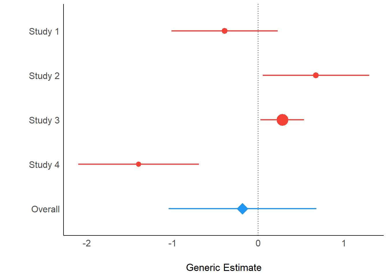
## Overall | -0.18 | 0.44 | [-1.05, 0.68] | -0.42 | 0.676 |Above you see the coefficients, their standard errors and the “weight”, based on the inverse variance. When you plot the results, the dot-geoms have different sizes, depending on the weight of the study (similar to metafor::forest()).
plot(result)
Check out more examples and documentation here (for parameters) and here (for see).
Get Involved
Note that easystats is a new project in active development, looking for contributors and supporters. Thus, do not hesitate to contact us if you want to get involved :)
- Check out our other blog posts here!
