Multilevel Correlations: A New Method for Common Problems

Apr 14, 2020 in CORRELATION • R
r easystats correlation
3 min read

In this tutorial, we will introduce multilevel correlations (or hierarchical / random-effects correlations) and how to compute them using the new correlations package from the easystats suite.

You can install the updated version and load the package as follows:

install.packages("correlation")
library(correlation)

Data

Imagine we have an experiment in which 10 individuals completed a task with 100 trials. For each of the 1000 total trials, we measured two things, V1 and V2, and our research aims at investingating the link between these two variables.

We will generate data using the simulate_simpson() function from the correlation package installed above.

data <- simulate_simpson(n=100, groups=10)

Now let’s visualize the two variables:

library(ggplot2)

ggplot(data, aes(x=V1, y=V2)) + 
  geom_point() +
  geom_smooth(colour="black", method="lm", se=FALSE) +
  theme_classic()

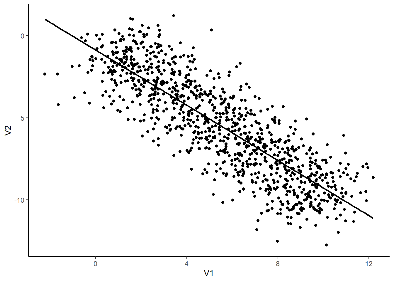
That seems pretty straightfoward! It seems like there is a negative correlation between V1 and V2. Let’s test this.

Simple correlation

correlation(data)

## Parameter1 | Parameter2 |     r |         95% CI | t(998) |      p |  Method | n_Obs
## ------------------------------------------------------------------------------------
## V1         |         V2 | -0.84 | [-0.86, -0.82] | -48.77 | < .001 | Pearson |  1000
## 
## p-value adjustment method: Holm (1979)

Indeed, there is strong, negative and significant correlation between V1 and V2. Great, can we go ahead and publish these results in PNAS?

The Simpson’s Paradox

Hold on sunshine! Ever heard of something called the Simpson’s Paradox?

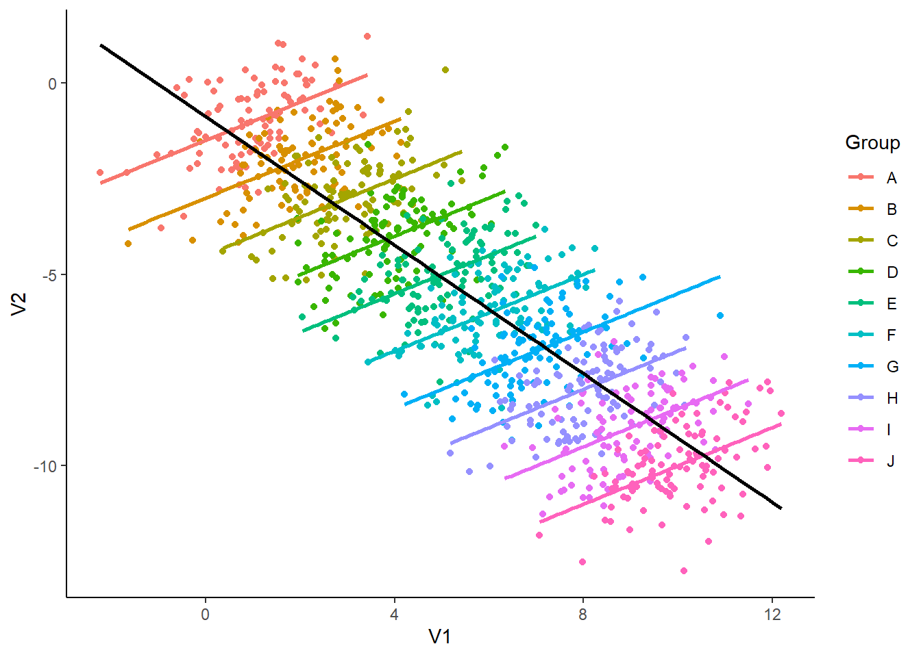
Let’s colour our datapoints by group (by individuals):

library(ggplot2)

ggplot(data, aes(x=V1, y=V2)) + 
  geom_point(aes(colour=Group)) +
  geom_smooth(aes(colour=Group), method="lm", se=FALSE) + 
  geom_smooth(colour="black", method="lm", se=FALSE) + 
  theme_classic()

Mmh, interesting. It seems like, for each subject, the relationship is different. The negative general trend seems to be created by differences between the groups and could be spurious!

Multilevel (as in multi-group) correlations allow us to account for differences between groups. It is based on a partialization of the group variable, entered as a random factor in a mixed linear regression.

You can compute them with the correlations package by setting the multilevel arguent to TRUE.

correlation(data, multilevel = TRUE)

## Parameter1 | Parameter2 |    r |           CI | t(998) |      p |  Method | n_Obs
## ---------------------------------------------------------------------------------
## V1         |         V2 | 0.50 | [0.45, 0.55] |  18.24 | < .001 | Pearson |  1000
## 
## p-value adjustment method: Holm (1979)

Dayum! We were too hasty in our conclusions! Taking the group into account seems to be super important.

Note: In this simple case where only two variables are of interest, it would be of course best to directly proceed using a mixed regression model instead of correlations. That being said, the latter can be useful for exploratory analysis, when multiple variables are of interest, or in combination with a network or structural approach.

Get Involved

easystats is a new project in active development, looking for contributors and supporters. Thus, do not hesitate to contact us if you want to get involved :)

Check out our other blog posts here!

Stay tuned

To be updated about the upcoming features and cool R or data science stuff, you can follow the packages on GitHub (click on one of the easystats package) and then on the Watch button on the top right corner) as well as the easystats team on twitter and online: