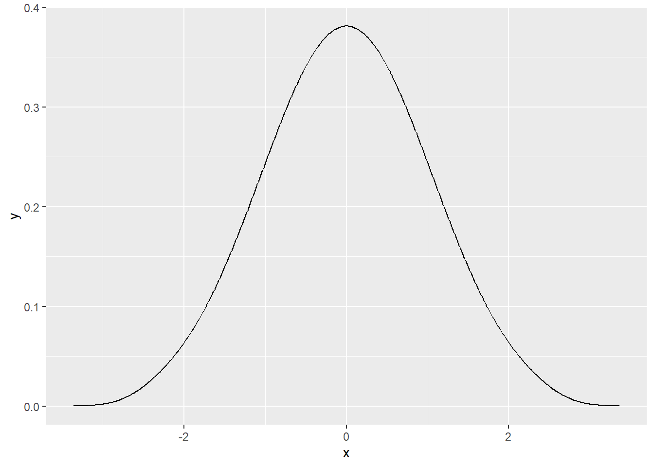
Many times, for instance when teaching, I needed to quickly and simply generate a perfectly normally distributed sample to illustrate or show some of its characteristics.
This is now very easy to do with the new bayestestR package, which includes the rnorm_perfect function. This function is very similar to the classic rnorm (same arguments), with the difference that the generated sample is perfectly normal.
Example
bayestestR can be installed as follows:
install.packages("bayestestR")  # Install the package
library(bayestestR)  # Load it
# Generate a perfect sample
x <- rnorm_perfect(n = 100, mean = 0, sd = 1)
# Visualise it
library(tidyverse)
x %>%
density() %>% # Compute density function
as.data.frame() %>%
ggplot(aes(x=x, y=y)) +
geom_line()
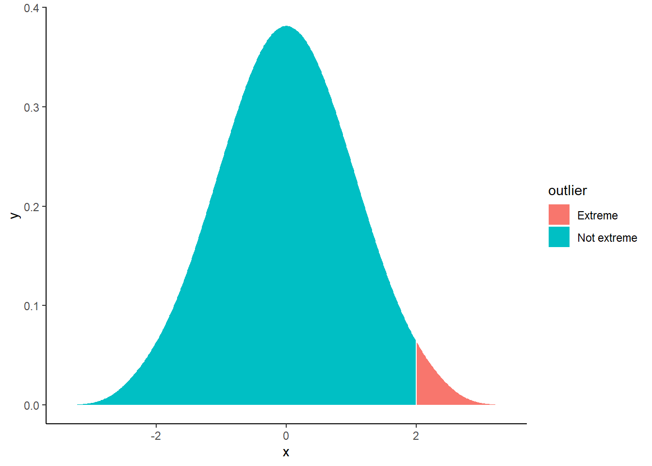
We can also easily color some of the parts of the curve, for instance, the observations lying beyond +2 standard deviations.
x %>%
  density() %>%  # Compute density function
  as.data.frame() %>%
  mutate(outlier = ifelse(x > 2, "Extreme", "Not extreme")) %>%
  ggplot(aes(x=x, y=y, fill=outlier)) +
  geom_ribbon(aes(ymin=0, ymax=y)) +
  theme_classic()
bayestestR and easystats
More details about bayestestR’s features are comming soon, stay tuned ;)
- Don’t forget to check out the documentation here for more!
Feel free to let us know how we could further improve this package! Also, note that easystats, the project supporting bayestestR is in active development. Thus, do not hesitate to contact us if you want to get involved :)
- Check out our other blog posts here!
